Chapter 10 One-Way ANOVA
Next, let’s go over the one-way ANOVA, which is used when we have two or more independent groups. Specifically, the one-way ANOVA determines if there is a difference in any of the group level means. Given that the analysis can also be used for two independent groups, this analysis could be used instead of the Independent Samples t-Test.
For example, let’s say that we were interested in determining if salary was significantly different for professors of different ranks (i.e., assistant professor, associate professor, and professor).
For this example, we will use the dataset: Salaries Dataset.
As mentioned in the Independent Samples t-Test, when dealing with categorical predictors, it is always a good idea to check the coding scheme of the categorical variable.
contrasts(datasetSalaries$rank)
##                     2 3
## Assistant Professor 0 0
## Associate Professor 1 0
## Professor           0 1
Section 10.1 Coding Categorical Variables
When coding categorical variables, the number of contrasts (\(m\)) is equal to \(k-1\) where \(k\) is the number of levels (or factors) of an IV. In our example,
rank has 3 levels (i.e., Assistant Professor, Associate Professor, and Professor) and thus has 2 contrasts.1
\(m_{rank} = k_{rank} - 1 = 3 - 1 = 2\)
This is the reason why in a one-way ANOVA, we have \(k-1\) between degrees of freedom. Thus, contrasts are always being performed, either explicitly if told or using a software package’s default coding scheme (e.g., dummy coding for R) when testing a main effect of a categorical IV.
Subsection 10.1.1 Dummy Coding
Since
rank has not yet been explicitly defined by us, rank is dummy coded (i.e., for each contrast, a level is coded as 1 and all other levels are coded as 0). In dummy coding, one level will always be coded as 0 in both contrasts. By default, the first level of the categorical IV in alphabetical order will be coded as 0. Thus, in our example, Assistant Professor, which is the first level of rank in alphabetical order, is coded as 0.
When interpreting dummy coding contrasts, for each contrast, it is the level that is coded as 1 compared to the level that is coded as 0 in both contrasts. In our dummy coding scheme, the first contrast is comparing
Associate Professor, which is coded as 1 in the first contrast, to Assistant Professor, which is coded as 0 in both contrasts. The second contrast is comparing Professor, which is coded as 1 in the second contrast, to Assistant Professor, which is again coded as 0 in both contrasts.
Subsection 10.1.2 Orthogonal Coding
However, a priori orthogonal contrast coding is preferred because this coding scheme allows us to create our own a priori contrasts of interest to answer more specific questions.
For example, let’s say that in addition to determining if there is a difference in salary of professors based on their rank, we were also interested in more specific questions of interest such as:
-
Determining if there is a difference in salaries of professors that are tenured (
Associate ProfessorandProfessor) compared to those that are untenured (Assistant Professor). -
Determining if there is a difference in salaries of professors that are
Associate Professorscompared toProfessors.
contrasts(datasetSalaries$rank) <- cbind(
  TenuredvAssistant = c(-2, 1, 1),
  AssociatevProfessor = c(0, -1, 1)
)
To make a coding scheme orthogonal, we need to make sure that 1) the sum of each contrast equals zero and that 2) the sum of each contrast product is 0.
For example, to make the tenured vs. untenured professor contrast, we can code
Assistant Professor as -2 and both Associate Professor and Professor as 1 and assign it the name TenuredvAssistant. It’s best to use signs that go in the direction of our prediction so that it’s reflected in our estimates. Since we expect that tenured professors have higher salaries, tenured professors are assigned the positive value and assistant professors are assigned the negative value. Notice that the sum of the TenuredvAssistant contrast also adds up to 0.2
\(\Sigma Contrast\_Codes_{TenuredvAssistant} = -2 + 1 + 1 = 0\)
To make the next contrast of
Associate Professor compared to Professor, we can code Assistant Professor as 0, Associate Professor as -1, and Professor as 1 and give it the name AssociatevProfessor. Notice again that the sum of the AssociatevProfessor contrast adds up to 0.3
\(\Sigma Contrast\_Code_{AssociatevProfessor} = 0 - 1 + 1 = 0\)
Since both contrasts sum to zero, we can now check if the sum of products for each level across contrasts equals 0. In other words, we multiply the values across each contrast pair for each level and add them together. For example, the product across the contrasts of
Assistant Professor is \(-2 \times 0 = 0\text{,}\) Associate Professor is \(1 \times -1 = -1\text{,}\) and Professor is \(1 \times 1 = 1\text{.}\) If we add them together, we get \(0 - 1 + 1 = 0\text{.}\)4
\(\Sigma Contrast_{TenuredvAssistant} \times Contrast_{AssociatevProfessor} = (-2 \times 0) + (1 \times -1) + (1 \times 1) = 0\)
To take orthogonal contrast coding a step further and make our estimates readily interpretable as the mean difference of that contrast, we can ensure that the difference of each contrast is 1. To do this, we can divide each contrast code by the number of values that are not coded as 0 for each contrast. For example, since all 3 codes of the
TenuredvAssistant contrast are not equal to 0, we can divide by 3. Similarly, for the AssociatevProfessor contrast, we can divide each contrast code by 2 since 2 of the contrast codes are not equal to 0. Note that this is a rule of thumb and should be verified if contrasts are more complex.
contrasts(datasetSalaries$rank) <- cbind(
  TenuredvAssistant = c(-2 / 3, 1 / 3, 1 / 3),
  AssociatevProfessor = c(0, -1 / 2, 1 / 2)
)
contrasts(datasetSalaries$rank)
##                     TenuredvAssistant AssociatevProfessor
## Assistant Professor        -0.6666667                 0.0
## Associate Professor         0.3333333                -0.5
## Professor                   0.3333333                 0.5
Section 10.2 Null and Research Hypotheses
Subsection 10.2.1 Traditional Approach
\begin{align*}
H_0\text{: } \mu_{Assistant\_Professors} \amp= \mu_{Associate\_Professors} = \mu_{Professors}\\
H_1\text{: } \mu_{Assistant\_Professors} \amp\ne \mu_{Associate\_Professors} \ne \mu_{Professors}\\
\amp\text{or } \mu_{Assistant\_Professors} \ne \mu_{Associate\_Professors} = \mu_{Professors}\\
\amp\text{or } \mu_{Assistant\_Professors} \ne \mu_{Professors} = \mu_{Associate\_Professors}\\
\amp\text{or } \mu_{Associate\_Professors} \ne \mu_{Professors} = \mu_{Assistant\_Professors}
\end{align*}
The null hypothesis states that there is no difference in salaries between professors of different ranks. The research hypothesis states that the salary of at least one rank of professors is different than the others. Thus, there are multiple options for a research hypothesis.
Subsection 10.2.2 GLM Approach
\begin{align*}
\text{Model: } Salary \amp= \beta_0 + \beta_1 \cdot TenuredvAssistant + \beta_2 \cdot AssociatevProfessor + \varepsilon\\
H_0\text{: } \beta_1 \amp= \beta_2 = 0\\
H_1\text{: } \beta_1 \amp\ne 0 \text{ and/or } \beta_2 \ne 0
\end{align*}
In the model, we now have both contrasts as predictors. The main effect of rank is testing both predictors of
TenuredvAssistant and AssociatevProfessor.
Given our orthogonal contrast coding scheme, the intercept (\(\beta_0\)) is now the mean 9-month academic salary of professors on average across rank.
The slope of
TenuredvAssistant (\(\beta_1\)) represents the mean difference in the 9-month academic salary for professors that are tenured compared to assistant professors.
The slope of
AssociatevProfessor (\(\beta_2\)) represents the mean difference in the 9-month academic salary for professors that are associate professors compared to professors.
Thus, the null hypothesis states that there is no difference in salary of tenured versus untenured professors and there is also no difference in salary of associate professors compared to professors. In other words, there is no difference in salary based on a professor’s rank. The alternative hypothesis states that there is a difference in either the salary of tenured versus untenured professors or associate professor versus professor, or both. If only one contrast is significant, then that contrast must be strong enough to mask the non-significance of the other contrast.
Given the vagueness of the research hypothesis (i.e., the significance can be a single contrast or both contrasts), we can look at each individual slope to see which is actually significant since we explicitly defined its associated contrasts beforehand.
Thus, our null and research hypotheses for these specific questions would be the following for each slope:
\begin{align*}
H_0\text{: } \beta_1 \amp= 0\\
H_1\text{: } \beta_1 \amp\ne 0\\
H_0\text{: } \beta_2 \amp= 0\\
H_1\text{: } \beta_2 \amp\ne 0
\end{align*}
Each of these null and research hypothesis pairs are also known as 1 degree of freedom tests since we are only testing 1 contrast at a time.
Section 10.3 Statistical Analysis
Subsection 10.3.1 Traditional Approach
To perform a traditional One-Way ANOVA, we can use the
aov() function. The first argument in the aov() function is the formula and the second argument is the name of the dataset. Notice that in the formula, we do not have to specify both contrasts because we have already applied the coding scheme directly to the categorical IV of rank.
model <- aov(salary ~ rank, datasetSalaries)
Anova(model, type = c("III"))
## Anova Table (Type III tests)
##
## Response: salary
##                 Sum Sq  Df F value    Pr(>F)
## (Intercept) 2.6481e+12   1 4741.08 < 2.2e-16 ***
## rank        1.4323e+11   2  128.22 < 2.2e-16 ***
## Residuals   2.2007e+11 394
## ---
## Signif. codes:  0 '***' 0.001 '**' 0.01 '*' 0.05 '.' 0.1 ' ' 1
Traditionally, if the main effect of a categorical IV was significant, we would perform a post-hoc test (e.g., Tukey’s Honest Significant Difference [HSD]). In our case,
rank is significant as the p-value of 2.2e-16 is less than our alpha of 0.05 and we would perform a post-hoc test to determine where the difference in salary actually comes from.
To perform Tukey’s HSD, we could use the
TukeyHSD function and provide the ANOVA analysis of the model as the input. The Tukey HSD essentially performs multiple independent samples t-tests of all possible pairs of the levels of a categorical IV but uses the error term from the ANOVA analysis in its calculation.
TukeyHSD(model)
##   Tukey multiple comparisons of means
##     95% family-wise confidence level
##
## Fit: aov(formula = salary ~ rank, data = datasetSalaries)
##
## $rank
##                                             diff       lwr      upr     p adj
## Associate Professor-Assistant Professor 13100.45  3382.195 22818.71 0.0046514
## Professor-Assistant Professor           45996.12 38395.941 53596.31 0.0000000
## Professor-Associate Professor           32895.67 25154.507 40636.84 0.0000000
Given that this post-hoc test compares all pairs of levels without any a priori assumptions (similarly, for other post-hoc tests), this is another reason to use the a priori orthogonal contrast coding scheme.
Subsection 10.3.2 GLM Approach
Notice that in the formula, we do not have to specify both contrasts because we have already applied the coding scheme directly to the categorical IV of
rank.
model <- lm(salary ~ 1 + rank, datasetSalaries)
Anova(model, type = c("III"))
## Anova Table (Type III tests)
##
## Response: salary
##                 Sum Sq  Df F value    Pr(>F)
## (Intercept) 2.6481e+12   1 4741.08 < 2.2e-16 ***
## rank        1.4323e+11   2  128.22 < 2.2e-16 ***
## Residuals   2.2007e+11 394
## ---
## Signif. codes:  0 '***' 0.001 '**' 0.01 '*' 0.05 '.' 0.1 ' ' 1
Note that in both analyses, the F-statistic of
128.22 with 2 between degrees of freedom (df), 394 within degrees of freedom (df), and p-value of 2.2e-16 are identical.
summary(model)
##
## Call:
## lm(formula = salary ~ 1 + rank, data = datasetSalaries)
##
## Residuals:
##    Min     1Q Median     3Q    Max
## -68972 -16376  -1580  11755 104773
##
## Coefficients:
##                         Estimate Std. Error t value Pr(>|t|)
## (Intercept)               100475       1459  68.855   <2e-16 ***
## rankTenuredvAssistant      29548       3323   8.892   <2e-16 ***
## rankAssociatevProfessor    32896       3290   9.997   <2e-16 ***
## ---
## Signif. codes:  0 '***' 0.001 '**' 0.01 '*' 0.05 '.' 0.1 ' ' 1
##
## Residual standard error: 23630 on 394 degrees of freedom
## Multiple R-squared:  0.3943, Adjusted R-squared:  0.3912
## F-statistic: 128.2 on 2 and 394 DF,  p-value: < 2.2e-16
The estimate for the
(Intercept) represents the mean 9-month academic salary on average across rank.
The estimate for the
rankTenuredvAssistant represents the mean difference in 9-month academic salary of tenured professors compared to assistant professors. Specifically, the 9-month academic salary of tenured professors was $29,548 more than assistant professors.
The estimate for the
rankAssociatevProfessor represents the mean difference in 9-month academic salary of associate professors compared to professors. Specifically, the 9-month academic salary of professors was $32,896 more than associate professors.
Section 10.4 Statistical Decision
Given the p-value of
< 2.2e-16 for rank is less than the alpha level (\(\alpha\)) of 0.05, we will reject the null hypothesis.
Notice both slopes are also significant, and we will also reject the null hypothesis for each.
Section 10.5 APA Statement
An Analysis of Variance (ANOVA) using a priori orthogonal contrast coding was performed to test if there was a difference in the 9-month academic salary between 1) tenured (i.e., associate professors and professors) compared to untenured professors (i.e., assistant professors) and 2) associate professors compared to professors. There was a significant main effect of rank on salary, F(2, 394) = 128.22, p < .001. Specific to our contrasts, tenured professors earned significantly more than untenured professors, b = $29,548, t(1, 394) = 8.892, p < .001. Professors also earned significantly more than associate professors, b = $32,896, t(1, 394) = 9.997, p < .001.
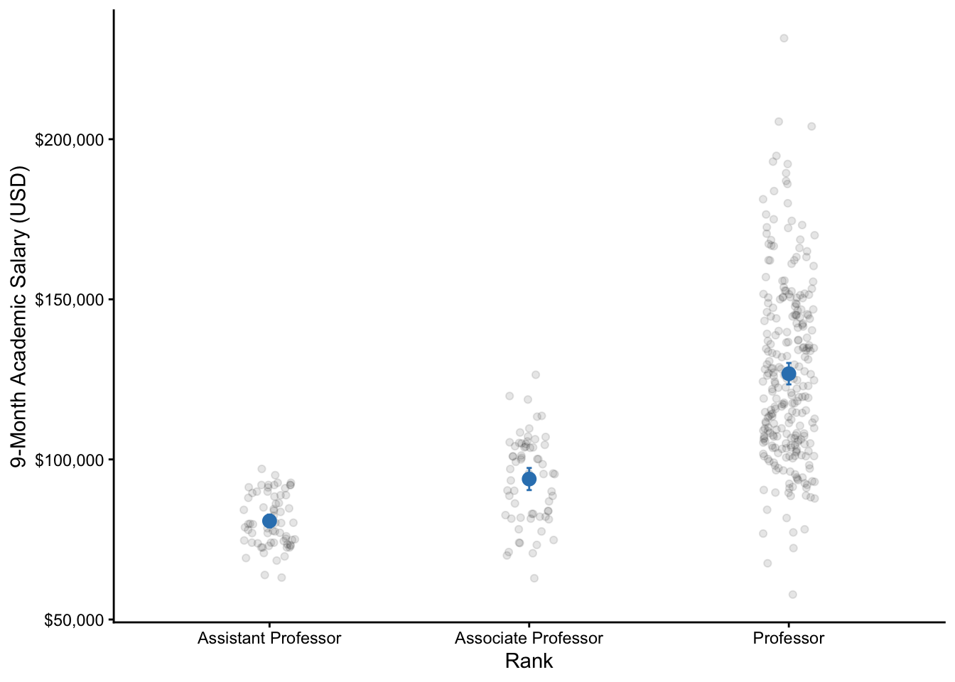
Section 10.6 Visualization
Subsection 10.6.1 Traditional
# calculate descriptive statistics along with the 95% CI
dataset_summary <- datasetSalaries %>%
  group_by(rank) %>%
  summarize(
    mean = mean(salary),
    sd = sd(salary),
    n = n(),
    sem = sd / sqrt(n),
    tcrit = abs(qt(0.05 / 2, df = n - 1)),
    ME = tcrit * sem,
    LL95CI = mean - ME,
    UL95CI = mean + ME
  )

# plot
ggplot(datasetSalaries, aes(rank, salary)) +
  geom_jitter(alpha = 0.1, width = 0.1) +
  geom_errorbar(data = dataset_summary, aes(x = rank, y = mean, ymin = LL95CI, ymax = UL95CI), color = "#3182bd", width = 0.02) +
  geom_point(dat = dataset_summary, aes(x = rank, y = mean), color = "#3182bd", size = 3) +
  labs(
    x = "Rank",
    y = "9-Month Academic Salary (USD)"
  ) +
  scale_y_continuous(labels = scales::dollar) +
  theme_classic()
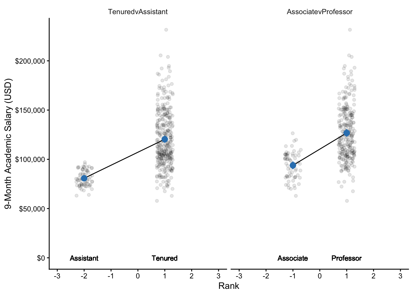
Subsection 10.6.2 Orthogonal Contrast Coding
datasetSalaries_long <- datasetSalaries %>%
  mutate(professor = 1:nrow(.),
         TenuredvAssistant = case_when(
    rank == "Assistant Professor" ~ -2,
    rank == "Associate Professor" ~ 1,
    rank == "Professor" ~ 1),
        AssociatevProfessor = case_when(
    rank == "Assistant Professor" ~ 0,
    rank == "Associate Professor" ~ -1,
    rank == "Professor" ~ 1)
  ) %>%
  select(professor, salary, TenuredvAssistant, AssociatevProfessor) %>%
  reshape2::melt(., id.vars = c("professor", "salary")) %>%
  filter(value != 0) %>%
  rowwise() %>%
  mutate(rank = case_when(
    variable == "TenuredvAssistant" && value == -2 ~ "Assistant",
    variable == "TenuredvAssistant" && value == 1 ~ "Tenured",
    variable == "AssociatevProfessor" && value == 1 ~ "Professor",
    variable == "AssociatevProfessor" && value == -1 ~ "Associate"
  ))

dataset_summary <- datasetSalaries_long %>%
  group_by(variable, value) %>%
  summarize(
    mean = mean(salary),
    sd = sd(salary),
    n = n(),
    sem = sd / sqrt(n),
    tcrit = abs(qt(0.05 / 2, df = n - 1)),
    ME = tcrit * sem,
    LL95CI = mean - ME,
    UL95CI = mean + ME
  )

ggplot(datasetSalaries_long, aes(value, salary)) +
  geom_jitter(alpha = 0.1, width = 0.3) +
  geom_errorbar(data = dataset_summary, aes(x = value, y = mean, ymin = LL95CI, ymax = UL95CI), color = "#3182bd", width = 0.05) +
  geom_line(data = dataset_summary, aes(x = value, y = mean)) +
  geom_point(data = dataset_summary, aes(x = value, y = mean), color = "#3182bd", size = 3) +
  geom_text(aes(label = rank, x = value, y = 0), size = 3) +
  facet_wrap(~ variable) +
  labs(
    x = "Rank",
    y = "9-Month Academic Salary (USD)"
  ) +
  scale_y_continuous(labels = scales::dollar) +
  scale_x_continuous(breaks = seq(-3, 3, 1), limits = c(-3,3)) +
  theme_classic() +
  theme(strip.background = element_blank())