Question: Interpret the confidence interval.
Answer.
Answer:
Solution.
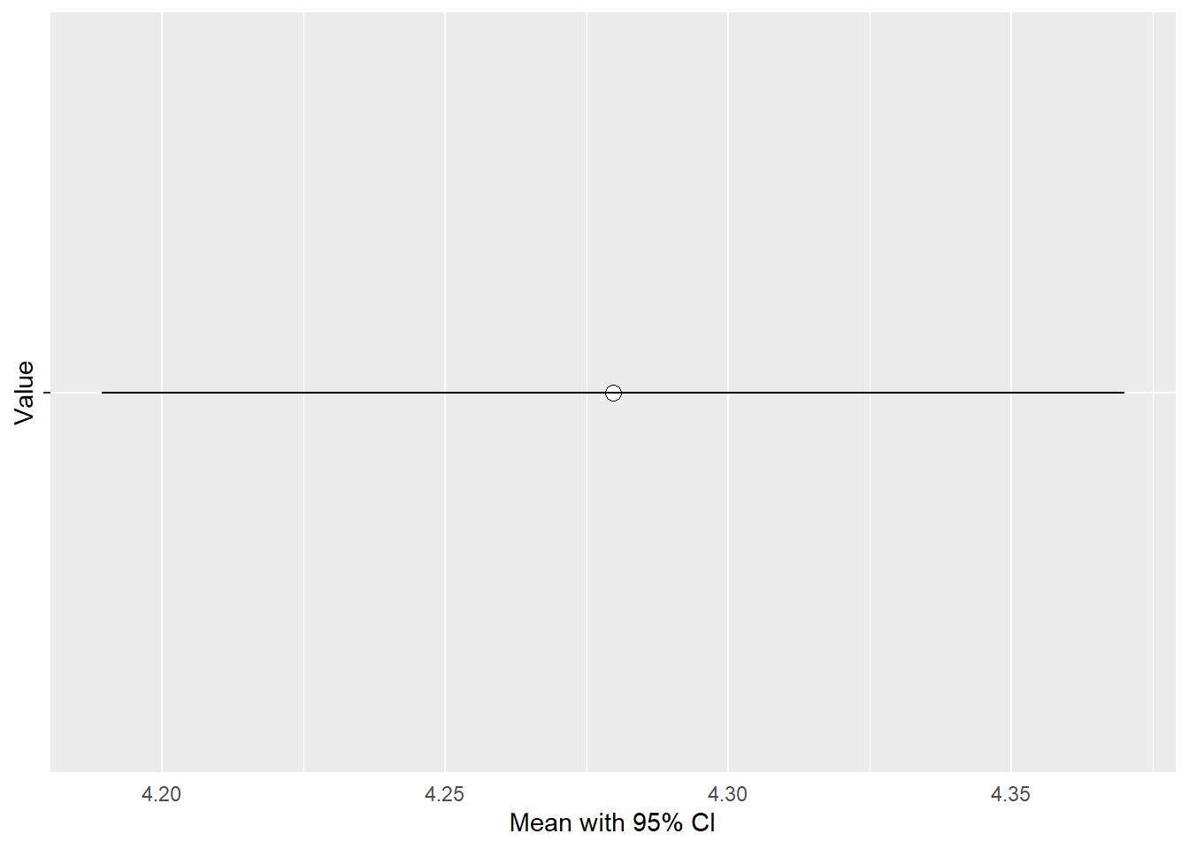
Interpretation: Likely values for the population mean are within the limits of 4.2 and 4.4.

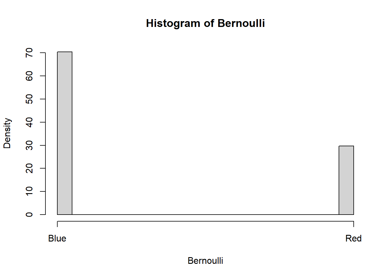
possible_values <- c(1,0)
Bernoulli <- sample(possible_values,
               size=10000,
               replace=TRUE,
               prob=c(0.3, 0.7))
prop.table(table(Bernoulli))
## Bernoulli
##      0      1
## 0.7034 0.2966
h <- hist(Bernoulli,plot=FALSE)
h$density = h$counts/sum(h$counts)*100
plot(h,freq=FALSE, axes=FALSE)
axis(1, at = c(0, 1), labels = c("Blue", "Red"))
axis(2, at = c(0, 10, 20, 30, 40, 50, 60, 70))
# Draw a standard normal distribution:
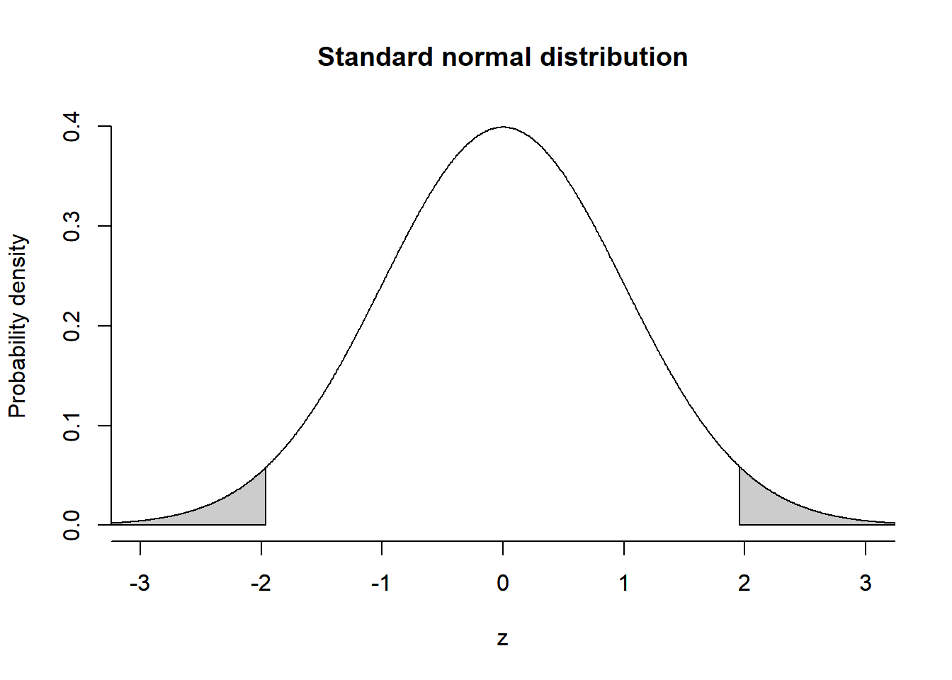
z = seq(-4, 4, length.out=1001)
x = rnorm(z)
plot( x=z, y=dnorm(z), bty='n', type='l', main="Standard normal distribution", ylab="Probability density", xlab="z", xlim=c(-3,3))
axis(1, at = seq(-4, 4, by = 1))

# annotate the density function with the 5% probability mass tails
polygon(x=c(z[z<=qnorm(0.025)], qnorm(0.025), min(z)), y=c(dnorm(z[z<=qnorm(0.025)]), 0, 0), col=grey(0.8))
polygon(x=c(z[z>=qnorm(0.975)], max(z), qnorm(0.975)), y=c(dnorm(z[z>=qnorm(0.975)]), 0, 0), col=grey(0.8))
set.seed(123)
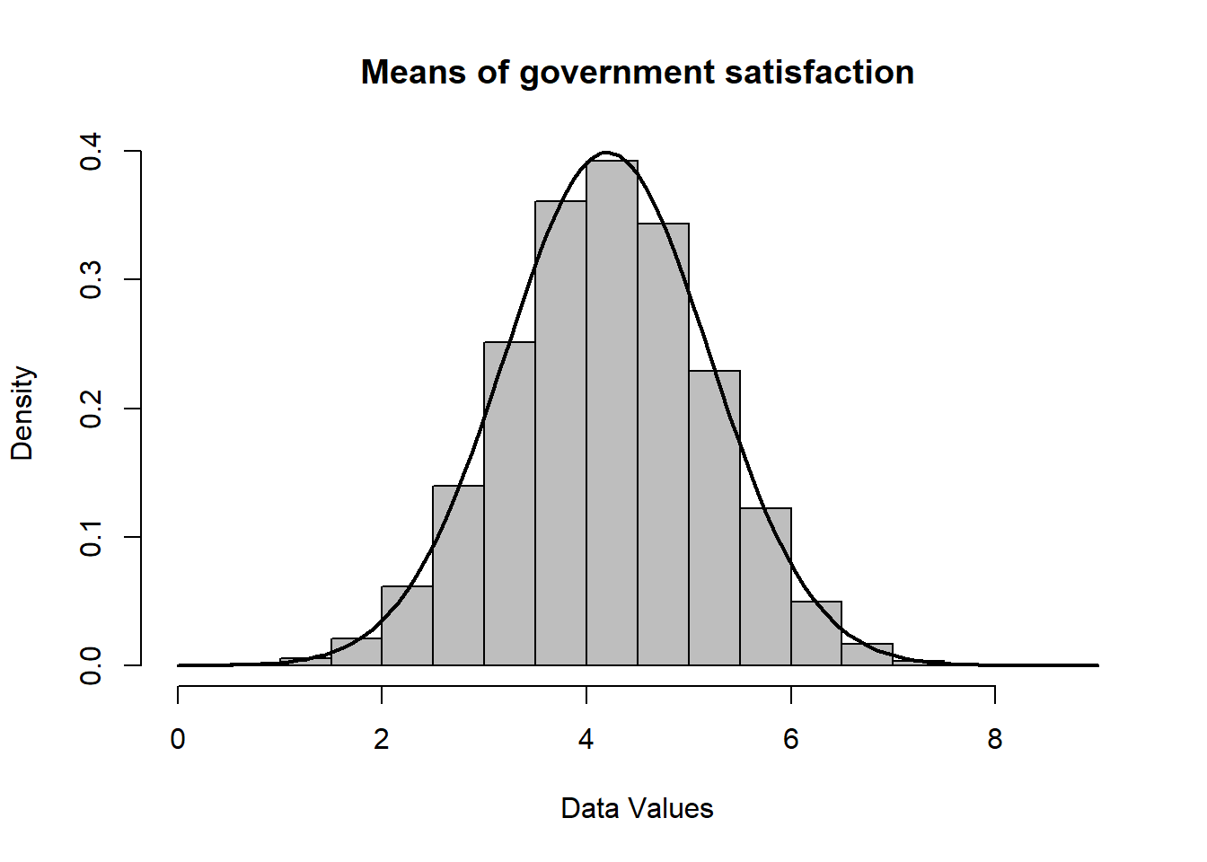
data <- rnorm(100000, 4.2, 1)
hist(data, freq = FALSE, col = "gray", xlab = "Data Values", main = "Means of government satisfaction")
curve(dnorm(x, mean = mean(data), sd = sd(data)), col = "black", lwd = 2, add = TRUE)
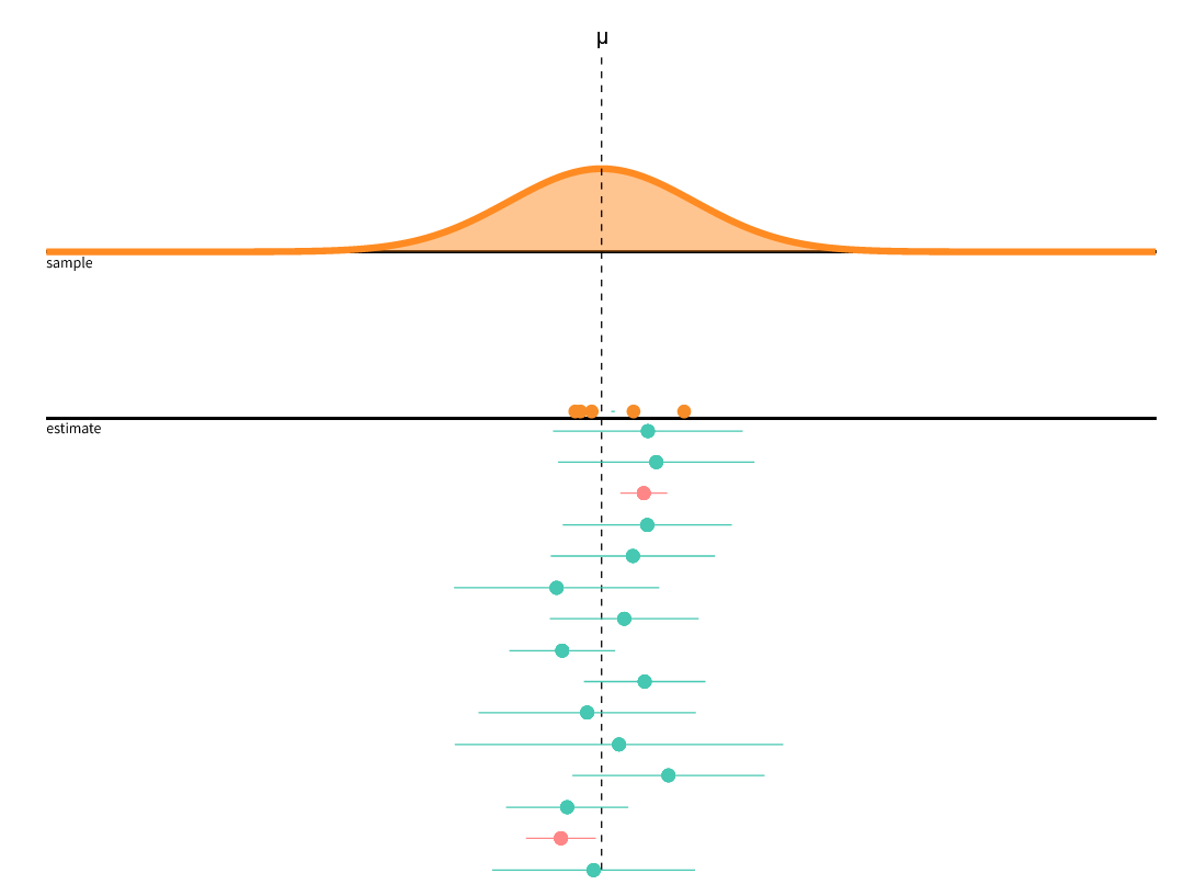
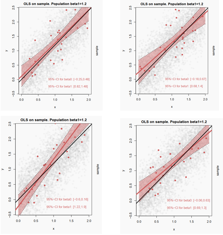
stfgov. stfgov was surveyed using an 11-point scale ranging from 0 "extremely dissatisfied" to 10 "extremely satisfied."
data_ess <- read_dta("data/ESS9_DE.dta", encoding = "latin1")

hist(data_ess$stfgov, breaks = "FD")

summary(data_ess$stfgov)
##    Min. 1st Qu.  Median    Mean 3rd Qu.    Max.    NA's
##    0.00    3.00    4.00    4.28    6.00   10.00      66
# We store the mean, the standard deviation and the number of observations as objects, because this way we can refer to them later on
n <- 2292
xbar <- mean(data_ess$stfgov, na.rm = TRUE)
s <- sd(data_ess$stfgov, na.rm = TRUE)

# Set confidence level with 1-alpha (alpha = our willingness to be wrong in repeated samples)
conf.level <- 0.95

# Calculating the critical z-value for a two-sided test
z <- qnorm((1 + conf.level) / 2)

# Calculate the confidence interval
lower.ci <- xbar - z * s / sqrt(n)
upper.ci <- xbar + z * s / sqrt(n)

# Print confidence intervals
cat("The", conf.level*100,"% confidence interval for the population mean is (",round(lower.ci, 2), ",", round(upper.ci, 2),").\n")
## The 95 % confidence interval for the population mean is ( 4.19 , 4.37 ).
t.test(data_ess$stfgov, conf.level = 0.95)
##
##  One Sample t-test
##
## data:  data_ess$stfgov
## t = 92.783, df = 2291, p-value < 2.2e-16
## alternative hypothesis: true mean is not equal to 0
## 95 percent confidence interval:
##  4.189216 4.370120
## sample estimates:
## mean of x
##  4.279668
df <- data.frame(xbar, lower.ci, upper.ci)

ggplot(df, aes(x = 1, y = xbar)) +
  theme(axis.text.y = element_blank(),
        axis.ticks.x = element_blank()) +
  geom_point(size = 3, shape = 21, fill = "white", colour = "black") +
  geom_errorbar(aes(ymin = lower.ci, ymax = upper.ci), width = 0.2) +
  coord_flip() +
  labs(x = "Value", y = "Mean with 95% CI") +
  scale_x_continuous(breaks = seq(0, 10, by = 1), limits = c(1, 1))
# Recode of variable
data_ess <- data_ess %>%
  mutate(stfgov_di =
           case_when(stfgov <= 5 ~ 0,
                     stfgov > 5 ~ 1))

# Proportion via table command
prop.table(table(data_ess$stfgov_di))
##        0        1
## 0.693281 0.306719
# Correspondence with the mean of the summary command
summary(data_ess$stfgov_di)
##    Min. 1st Qu.  Median    Mean 3rd Qu.    Max.    NA's
##  0.0000  0.0000  0.0000  0.3067  1.0000  1.0000      66
# Set confidence level with 1-alpha
conf.level <- 0.95

# Calculating the critical z-value for a two-sided test
z <- qnorm((1 + conf.level) / 2)

# Calculation of the confidence interval
lower.ci <- 0.3067 - z * sqrt((0.3067*(1-0.3067))/n)
upper.ci <- 0.3067 + z * sqrt((0.3067*(1-0.3067))/n)

# Print the confidence intervals
cat("The", conf.level*100, "% confidence interval for the proportion value is (", round(lower.ci, 2), ",", round(upper.ci, 2), ").\n")
## The 95 % confidence interval for the proportion value is ( 0.29 , 0.33 ).
# Test using t.test
t.test(data_ess$stfgov_di, conf.level = 0.95)
##
##  One Sample t-test
##
## data:  data_ess$stfgov_di
## t = 31.837, df = 2291, p-value < 2.2e-16
## alternative hypothesis: true mean is not equal to 0
## 95 percent confidence interval:
##  0.2878265 0.3256115
## sample estimates:
## mean of x
##  0.306719
hinctnta measures respondents’ net household income (after deductions) across 10 quantiles ("deciles" 1-10) - the reason for this measurement is that this way income becomes adjusted to a country’s income distribution and is thus comparable across countries. Regarding the correlation, we assume that - in line with economic voting theory - people with a higher income are more satisfied with the government than people with a lower income.
cor <- cor.test(data_ess$hinctnta, data_ess$stfgov)
cor
##
##  Pearson's product-moment correlation
##
## data:  data_ess$hinctnta and data_ess$stfgov
## t = 1.805, df = 2047, p-value = 0.07122
## alternative hypothesis: true correlation is not equal to 0
## 95 percent confidence interval:
##  -0.003445968  0.083023781
## sample estimates:
##        cor
## 0.03986354
ciplot <- ggplot(data=data_ess, aes(x = hinctnta , y = stfgov)) +
  geom_smooth(method = lm, se = TRUE, level = 0.95) +
  xlab("Income (Deciles)") +
  ylab("Satisfaction with the government")
ciplot
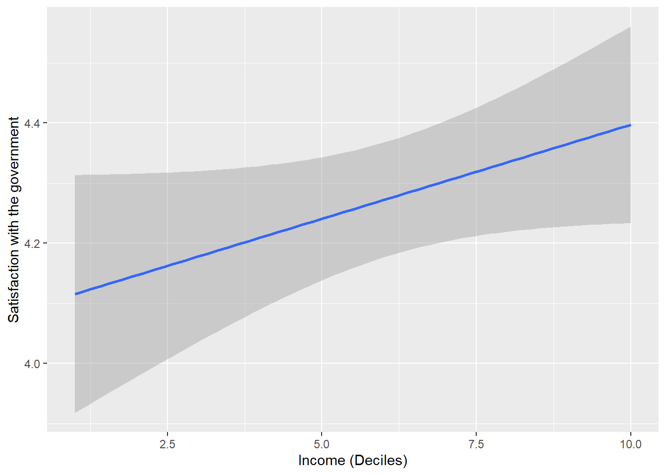
stfgov in its original metric form so that we can calculate the mean. However, we dichotomize the variable income hinctnta into two groups: low earners and high earners.
data_ess <- data_ess %>%
  mutate(hinctnta_di =
           case_when(hinctnta <= 6 ~ 0,
                     hinctnta > 6 ~ 1))
summary(data_ess$hinctnta_di)
##    Min. 1st Qu.  Median    Mean 3rd Qu.    Max.    NA's
##  0.0000  0.0000  0.0000  0.4794  1.0000  1.0000     270
# Draw a standard normal distribution:
z = seq(-4, 4, length.out=1001)
x = rnorm(z)

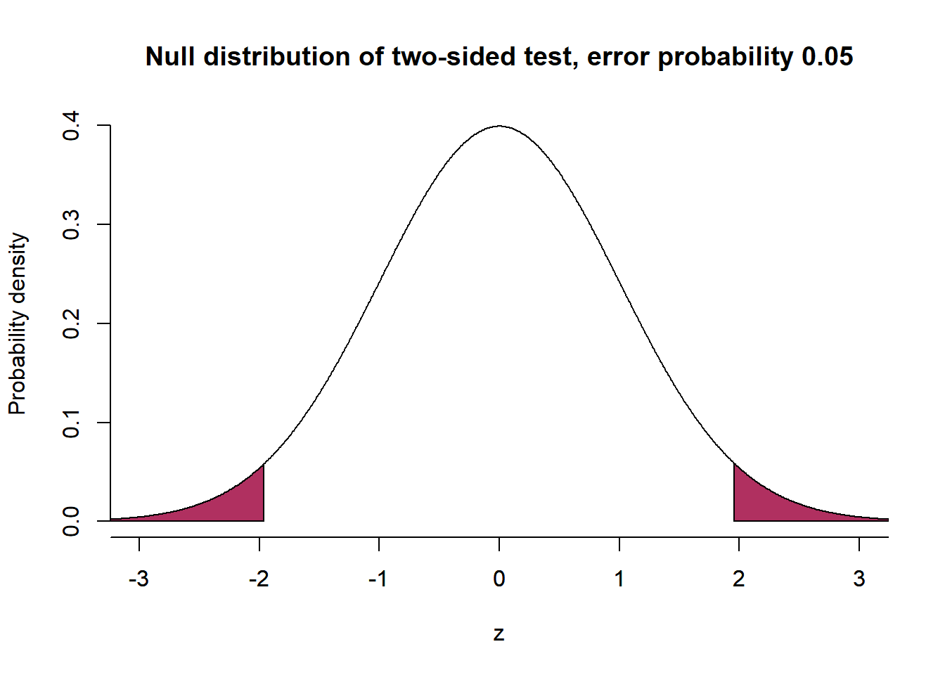
# Null distribution of two-sided test
plot( x=z, y=dnorm(z), bty='n', type='l', main="Null distribution of two-sided test, error probability 0.05", ylab="Probability density", xlab="z", xlim=c(-3,3))
axis(1, at = seq(-4, 4, by = 1))
polygon(x=c(z[z<=qnorm(0.025)], qnorm(0.025), min(z)), y=c(dnorm(z[z<=qnorm(0.025)]), 0, 0), col="maroon")
polygon(x=c(z[z>=qnorm(0.975)], max(z), qnorm(0.975)), y=c(dnorm(z[z>=qnorm(0.975)]), 0, 0), col="maroon")
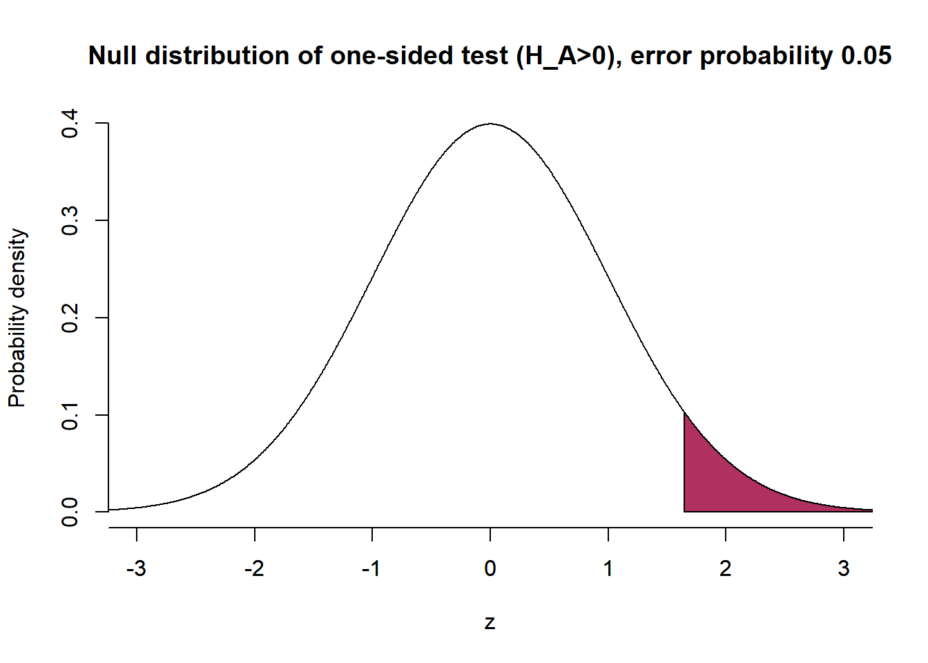
# Null distribution of one-sided test (H_A>0)
plot( x=z, y=dnorm(z), bty='n', type='l', main="Null distribution of one-sided test (H_A>0), error probability 0.05", ylab="Probability density", xlab="z", xlim=c(-3,3))
axis(1, at = seq(-4, 4, by = 1))
polygon(x=c(z[z>=qnorm(0.95)], max(z), qnorm(0.95)), y=c(dnorm(z[z>=qnorm(0.95)]), 0, 0), col="maroon")
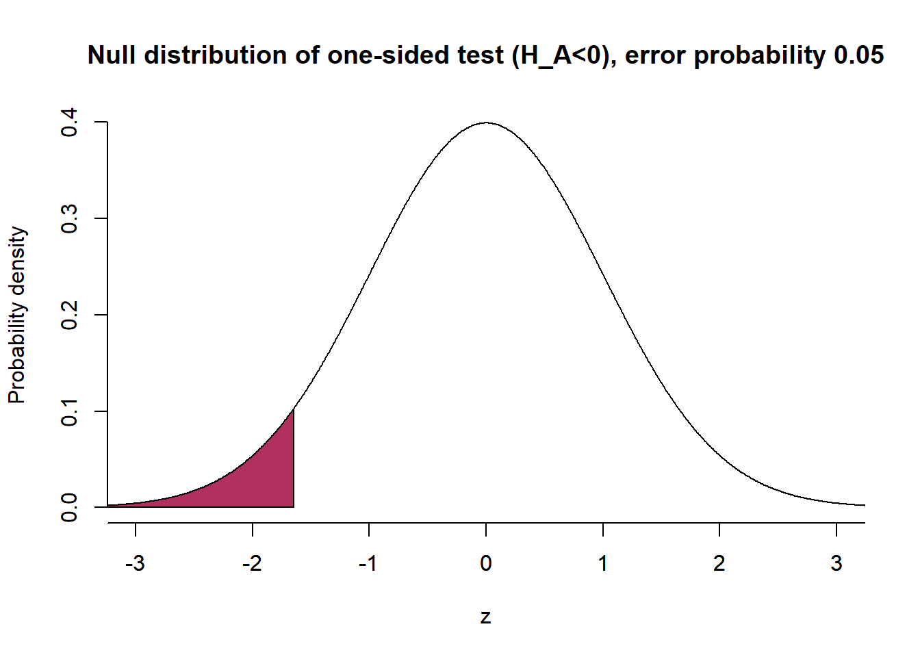
# Null distribution of one-sided test (H_A<0)
plot( x=z, y=dnorm(z), bty='n', type='l', main="Null distribution of one-sided test (H_A<0), error probability 0.05", ylab="Probability density", xlab="z", xlim=c(-3,3))
axis(1, at = seq(-4, 4, by = 1))
polygon(x=c(z[z<=qnorm(0.05)], qnorm(0.05), min(z)), y=c(dnorm(z[z<=qnorm(0.05)]), 0, 0), col="maroon")
mean(data_ess$stfgov[data_ess$hinctnta_di==1], na.rm = TRUE)-
  mean(data_ess$stfgov[data_ess$hinctnta_di==0], na.rm = TRUE)
## [1] 0.1543566
t.test(data_ess$stfgov[data_ess$hinctnta_di==1], data_ess$stfgov[data_ess$hinctnta_di==0])
##  Welch Two Sample t-test
##
## data:  data_ess$stfgov[data_ess$hinctnta_di == 1] and data_ess$stfgov[data_ess$hinctnta_di == 0]
## t = 1.5882, df = 2046.8, p-value = 0.1124
## alternative hypothesis: true difference in means is not equal to 0
## 95 percent confidence interval:
##  -0.03624397  0.34495717
## sample estimates:
## mean of x mean of y
##  4.354545  4.200189
cor <- cor.test(data_ess$hinctnta, data_ess$stfgov)
cor
##
##  Pearson's product-moment correlation
##
## data:  data_ess$hinctnta and data_ess$stfgov
## t = 1.805, df = 2047, p-value = 0.07122
## alternative hypothesis: true correlation is not equal to 0
## 95 percent confidence interval:
##  -0.003445968  0.083023781
## sample estimates:
##        cor
## 0.03986354