\t is an example of an escaped character, which always starts with a backslash (\). Escaped characters are used to represent non-printing characters (like the tab) or those with special meanings (such as quotation marks).
read_csv
read_tsv
read_csv2
read_delim
read_excel
read_* functions.
tidyverse read_* function and function arguments to load a given plain text tabular data set into R.
rename function to rename columns in a data frame.
read_excel function and arguments to load a sheet from an excel file into R.
dbplyr and DBI:dbConnect.
dbListTables.
tbl.
collect.
rvest package.
httr2 package.
.csv), accessing data from an API, and scraping the HTML source code from a website.
project3.ipynb, and our current working directory is project3; typically, as is the case here, the working directory is the directory containing the file you are currently working on.
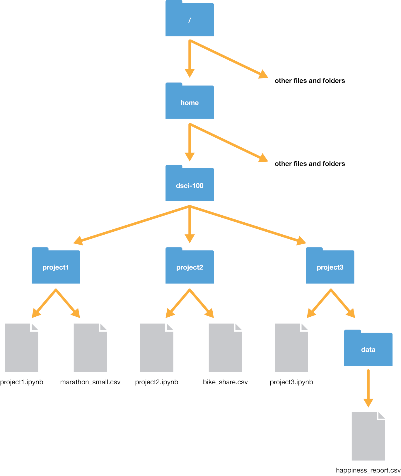
happiness_report.csv file. We have two options to indicate where the file is: using a relative path, or using an absolute path. The absolute path of the file always starts with a slash /—representing the root folder on the computer—and proceeds by listing out the sequence of folders you would have to enter to reach the file, each separated by another slash /. So in this case, happiness_report.csv would be reached by starting at the root, and entering the home folder, then the dsci-100 folder, then the project3 folder, and then finally the data folder. So its absolute path would be /home/dsci-100/project3/data/happiness_report.csv. We can load the file using its absolute path as a string passed to the read_csv function.
happy_data <- read_csv("/home/dsci-100/project3/data/happiness_report.csv")
/ separating each step. Since we are currently in the project3 folder, we just need to enter the data folder to reach our desired file. Hence the relative path is data/happiness_report.csv, and we can load the file using its relative path as a string passed to read_csv.
happy_data <- read_csv("data/happiness_report.csv")
"/data/happiness_report.csv", R would look for a folder named data in the root folder of the computer—but that doesn’t exist!
data and project3), we can also specify two additional special places: the current directory and the previous directory. We indicate the current working directory with a single dot ., and the previous directory with two dots ... So for instance, if we wanted to reach the bike_share.csv file from the project3 folder, we could use the relative path ../project2/bike_share.csv. We can even combine these two; for example, we could reach the bike_share.csv file using the (very silly) path ../project2/../project2/./bike_share.csv with quite a few redundant directions: it says to go back a folder, then open project2, then go back a folder again, then open project2 again, then stay in the current directory, then finally get to bike_share.csv. Whew, what a long trip!
/, and the file) isn’t usually the same across different computers. For example, suppose Fatima and Jayden are working on a project together on the happiness_report.csv data. Fatima’s file is stored at
/home/Fatima/project3/data/happiness_report.csv,
/home/Jayden/project3/data/happiness_report.csv.
happiness_report.csv data using an absolute path, the code won’t work on Fatima’s computer. But the relative path from inside the project3 folder (data/happiness_report.csv) is the same on both computers; any code that uses relative paths will work on both! In the additional resources section, we include a link to a short video on the difference between absolute and relative paths. You can also check out the here package, which provides methods for finding and constructing file paths in R.
/, and then a path to where the resource is located on the remote machine.
read_csv to read in comma-separated values files
tidyverse read_csv function when reading .csv (comma-separated values) files. In that case, the separator or delimiter that divided our columns was a comma (,). We only learned the case where the data matched the expected defaults of the read_csv function (column names are present, and commas are used as the delimiter between columns). In this section, we will learn how to read files that do not satisfy the default expectations of read_csv.
tidyverse and read_csv, let’s revisit the more straightforward case where the defaults hold, and the only argument we need to give to the function is the path to the file, data/can_lang.csv. The can_lang data set contains language data from the 2016 Canadian census. We put data/ before the file’s name when we are loading the data set because this data set is located in a sub-folder, named data, relative to where we are running our R code. Here is what the text in the file data/can_lang.csv looks like.
category,language,mother_tongue,most_at_home,most_at_work,lang_known
Aboriginal languages,"Aboriginal languages, n.o.s.",590,235,30,665
Non-Official & Non-Aboriginal languages,Afrikaans,10260,4785,85,23415
Non-Official & Non-Aboriginal languages,"Afro-Asiatic languages, n.i.e.",1150,445,10,2775
Non-Official & Non-Aboriginal languages,Akan (Twi),13460,5985,25,22150
Non-Official & Non-Aboriginal languages,Albanian,26895,13135,345,31930
read_csv to load it into R. First we load the tidyverse package to gain access to useful functions for reading the data.
library(tidyverse)
read_csv to load the data into R, and in that call we specify the relative path to the file. Note that it is normal and expected that a message is printed out after using the read_csv and related functions. This message lets you know the data types of each of the columns that R inferred while reading the data into R. In the future when we use this and related functions to load data in this book, we will silence these messages to help with the readability of the book.
canlang_data <- read_csv("data/can_lang.csv")
Rows: 214 Columns: 6
── Column specification ────────────────────────────────────────────────────────
Delimiter: ","
chr (2): category, language
dbl (4): mother_tongue, most_at_home, most_at_work, lang_known
ℹ Use `spec()` to retrieve the full column specification for this data.
ℹ Specify the column types or set `show_col_types = FALSE` to quiet this message.
canlang_data
# A tibble: 214 × 6
## # A tibble: 214 × 6
##    category          language mother_tongue most_at_home most_at_work lang_known
##    <chr>             <chr>            <dbl>        <dbl>        <dbl>      <dbl>
##  1 Aboriginal langu… Aborigi…           590          235           30        665
##  2 Non-Official & N… Afrikaa…         10260         4785           85      23415
##  3 Non-Official & N… Afro-As…          1150          445           10       2775
##  4 Non-Official & N… Akan (T…         13460         5985           25      22150
##  5 Non-Official & N… Albanian         26895        13135          345      31930
##  6 Aboriginal langu… Algonqu…            45           10            0        120
##  7 Aboriginal langu… Algonqu…          1260          370           40       2480
##  8 Non-Official & N… America…          2685         3020         1145      21930
##  9 Non-Official & N… Amharic          22465        12785          200      33670
## 10 Non-Official & N… Arabic          419890       223535         5585     629055
## # ℹ 204 more rows
Data source: https://ttimbers.github.io/canlang/
Data originally published in: Statistics Canada Census of Population 2016.
Reproduced and distributed on an as-is basis with their permission.
category,language,mother_tongue,most_at_home,most_at_work,lang_known
Aboriginal languages,"Aboriginal languages, n.o.s.",590,235,30,665
Non-Official & Non-Aboriginal languages,Afrikaans,10260,4785,85,23415
Non-Official & Non-Aboriginal languages,"Afro-Asiatic languages, n.i.e.",1150,44
Non-Official & Non-Aboriginal languages,Akan (Twi),13460,5985,25,22150
Non-Official & Non-Aboriginal languages,Albanian,26895,13135,345,31930
Aboriginal languages,"Algonquian languages, n.i.e.",45,10,0,120
Aboriginal languages,Algonquin,1260,370,40,2480
Non-Official & Non-Aboriginal languages,American Sign Language,2685,3020,1145,21
Non-Official & Non-Aboriginal languages,Amharic,22465,12785,200,33670
read_csv as we did previously does not allow us to correctly load the data into R. In the case of this file we end up only reading in one column of the data set. In contrast to the normal and expected messages above, this time R prints out a warning for us indicating that there might be a problem with how our data is being read in.
canlang_data <- read_csv("data/can_lang_meta-data.csv")
canlang_data
## Warning: One or more parsing issues, call `problems()` on your data frame for details,
## e.g.:
##   dat <- vroom(...)
##   problems(dat)

## # A tibble: 217 × 1
##    `Data source: https://ttimbers.github.io/canlang/`
##    <chr>
##  1 "Data originally published in: Statistics Canada Census of Population 2016."
##  2 "Reproduced and distributed on an as-is basis with their permission."
##  3 "category,language,mother_tongue,most_at_home,most_at_work,lang_known"
##  4 "Aboriginal languages,\"Aboriginal languages, n.o.s.\",590,235,30,665"
##  5 "Non-Official & Non-Aboriginal languages,Afrikaans,10260,4785,85,23415"
##  6 "Non-Official & Non-Aboriginal languages,\"Afro-Asiatic languages, n.i.e.\",…
##  7 "Non-Official & Non-Aboriginal languages,Akan (Twi),13460,5985,25,22150"
##  8 "Non-Official & Non-Aboriginal languages,Albanian,26895,13135,345,31930"
##  9 "Aboriginal languages,\"Algonquian languages, n.i.e.\",45,10,0,120"
## 10 "Aboriginal languages,Algonquin,1260,370,40,2480"
## # ℹ 207 more rows
skip argument can be useful to tell R how many lines to skip before it should start reading in the data. In the example above, we would set this value to 3.
canlang_data <- read_csv("data/can_lang_meta-data.csv",
                         skip = 3)
canlang_data
## # A tibble: 214 × 6
##    category          language mother_tongue most_at_home most_at_work lang_known
##    <chr>             <chr>            <dbl>        <dbl>        <dbl>      <dbl>
##  1 Aboriginal langu… Aborigi…           590          235           30        665
##  2 Non-Official & N… Afrikaa…         10260         4785           85      23415
##  3 Non-Official & N… Afro-As…          1150          445           10       2775
##  4 Non-Official & N… Akan (T…         13460         5985           25      22150
##  5 Non-Official & N… Albanian         26895        13135          345      31930
##  6 Aboriginal langu… Algonqu…            45           10            0        120
##  7 Aboriginal langu… Algonqu…          1260          370           40       2480
##  8 Non-Official & N… America…          2685         3020         1145      21930
##  9 Non-Official & N… Amharic          22465        12785          200      33670
## 10 Non-Official & N… Arabic          419890       223535         5585     629055
## # ℹ 204 more rows
Data source: https://ttimbers.github.io/canlang/
Data originally published in: Statistics Canada Census of Population 2016.
Reproduced and distributed on an as-is basis with their permission.
read_tsv to read in tab-separated values files
can_lang.tsv, has tabs in between the columns instead of commas.
category    language    mother_tongue   most_at_home    most_at_work    lang_kno
Aboriginal languages    Aboriginal languages, n.o.s.    590 235 30  665
Non-Official & Non-Aboriginal languages Afrikaans   10260   4785    85  23415
Non-Official & Non-Aboriginal languages Afro-Asiatic languages, n.i.e.  1150
Non-Official & Non-Aboriginal languages Akan (Twi)  13460   5985    25  22150
Non-Official & Non-Aboriginal languages Albanian    26895   13135   345 31930
Aboriginal languages    Algonquian languages, n.i.e.    45  10  0   120
Aboriginal languages    Algonquin   1260    370 40  2480
Non-Official & Non-Aboriginal languages American Sign Language  2685    3020
Non-Official & Non-Aboriginal languages Amharic 22465   12785   200 33670
canlang_data <- read_tsv("data/can_lang.tsv")
canlang_data
## # A tibble: 214 × 6
##    category          language mother_tongue most_at_home most_at_work lang_known
##    <chr>             <chr>            <dbl>        <dbl>        <dbl>      <dbl>
##  1 Aboriginal langu… Aborigi…           590          235           30        665
##  2 Non-Official & N… Afrikaa…         10260         4785           85      23415
##  3 Non-Official & N… Afro-As…          1150          445           10       2775
##  4 Non-Official & N… Akan (T…         13460         5985           25      22150
##  5 Non-Official & N… Albanian         26895        13135          345      31930
##  6 Aboriginal langu… Algonqu…            45           10            0        120
##  7 Aboriginal langu… Algonqu…          1260          370           40       2480
##  8 Non-Official & N… America…          2685         3020         1145      21930
##  9 Non-Official & N… Amharic          22465        12785          200      33670
## 10 Non-Official & N… Arabic          419890       223535         5585     629055
## # ℹ 204 more rows
read_csv, you’ll notice that they look identical: they have the same number of columns and rows, the same column names, and the same entries! So even though we needed to use a different function depending on the file format, our resulting data frame (canlang_data) in both cases was the same.
read_delim as a more flexible method to get tabular data into R
read_csv and read_tsv functions are actually just special cases of the more general read_delim function. We can use read_delim to import both comma and tab-separated values files, and more; we just have to specify the delimiter. For example, the can_lang_no_names.tsv file contains a different version of this same data set with no column names and uses tabs as the delimiter instead of commas. Here is how the file would look in a plain text editor:
Aboriginal languages    Aboriginal languages, n.o.s.    590 235 30  665
Non-Official & Non-Aboriginal languages Afrikaans   10260   4785    85  23415
Non-Official & Non-Aboriginal languages Afro-Asiatic languages, n.i.e.  1150
Non-Official & Non-Aboriginal languages Akan (Twi)  13460   5985    25  22150
Non-Official & Non-Aboriginal languages Albanian    26895   13135   345 31930
Aboriginal languages    Algonquian languages, n.i.e.    45  10  0   120
Aboriginal languages    Algonquin   1260    370 40  2480
Non-Official & Non-Aboriginal languages American Sign Language  2685    3020
Non-Official & Non-Aboriginal languages Amharic 22465   12785   200 33670
Non-Official & Non-Aboriginal languages Arabic  419890  223535  5585    629055
read_delim function, we specify the path to the file as the first argument, provide the tab character "\t" as the delim argument, and set the col_names argument to FALSE to denote that there are no column names provided in the data. Note that the read_csv, read_tsv, and read_delim functions all have a col_names argument with the default value TRUE.
\t is an example of an escaped character, which always starts with a backslash (\). Escaped characters are used to represent non-printing characters (like the tab) or those with special meanings (such as quotation marks).
canlang_data <- read_delim("data/can_lang_no_names.tsv",
                           delim = "\t",
                           col_names = FALSE)
canlang_data
## # A tibble: 214 × 6
##    X1                                      X2             X3     X4    X5     X6
##    <chr>                                   <chr>       <dbl>  <dbl> <dbl>  <dbl>
##  1 Aboriginal languages                    Aborigina…    590    235    30    665
##  2 Non-Official & Non-Aboriginal languages Afrikaans   10260   4785    85  23415
##  3 Non-Official & Non-Aboriginal languages Afro-Asia…   1150    445    10   2775
##  4 Non-Official & Non-Aboriginal languages Akan (Twi)  13460   5985    25  22150
##  5 Non-Official & Non-Aboriginal languages Albanian    26895  13135   345  31930
##  6 Aboriginal languages                    Algonquia…     45     10     0    120
##  7 Aboriginal languages                    Algonquin    1260    370    40   2480
##  8 Non-Official & Non-Aboriginal languages American …   2685   3020  1145  21930
##  9 Non-Official & Non-Aboriginal languages Amharic     22465  12785   200  33670
## 10 Non-Official & Non-Aboriginal languages Arabic     419890 223535  5585 629055
## # ℹ 204 more rows
X1, X2, X3, X4, X5, X6. It is best to rename your columns manually in this scenario. The current column names (X1, X2, etc.) are not very descriptive and will make your analysis confusing. To rename your columns, you can use the rename function from the dplyr R package [14] (one of the packages loaded with tidyverse, so we don’t need to load it separately). The first argument is the data set, and in the subsequent arguments you write new_name = old_name for the selected variables to rename. We rename the X1, X2, ..., X6 columns in the canlang_data data frame to more descriptive names below.
canlang_data <- rename(canlang_data,
       category = X1,
       language = X2,
       mother_tongue = X3,
       most_at_home = X4,
       most_at_work = X5,
       lang_known = X6)
canlang_data
## # A tibble: 214 × 6
##    category          language mother_tongue most_at_home most_at_work lang_known
##    <chr>             <chr>            <dbl>        <dbl>        <dbl>      <dbl>
##  1 Aboriginal langu… Aborigi…           590          235           30        665
##  2 Non-Official & N… Afrikaa…         10260         4785           85      23415
##  3 Non-Official & N… Afro-As…          1150          445           10       2775
##  4 Non-Official & N… Akan (T…         13460         5985           25      22150
##  5 Non-Official & N… Albanian         26895        13135          345      31930
##  6 Aboriginal langu… Algonqu…            45           10            0        120
##  7 Aboriginal langu… Algonqu…          1260          370           40       2480
##  8 Non-Official & N… America…          2685         3020         1145      21930
##  9 Non-Official & N… Amharic          22465        12785          200      33670
## 10 Non-Official & N… Arabic          419890       223535         5585     629055
## # ℹ 204 more rows
read_csv, read_tsv, or read_delim (and related functions) to read in data directly from a Uniform Resource Locator (URL) that contains tabular data. Here, we provide the URL of a remote file to read_*, instead of a path to a local file on our computer.
url <- "https://raw.githubusercontent.com/UBC-DSCI/data/main/can_lang.csv"
canlang_data <- read_csv(url)
canlang_data
## # A tibble: 214 × 6
##    category          language mother_tongue most_at_home most_at_work lang_known
##    <chr>             <chr>            <dbl>        <dbl>        <dbl>      <dbl>
##  1 Aboriginal langu… Aborigi…           590          235           30        665
##  2 Non-Official & N… Afrikaa…         10260         4785           85      23415
##  3 Non-Official & N… Afro-As…          1150          445           10       2775
##  4 Non-Official & N… Akan (T…         13460         5985           25      22150
##  5 Non-Official & N… Albanian         26895        13135          345      31930
##  6 Aboriginal langu… Algonqu…            45           10            0        120
##  7 Aboriginal langu… Algonqu…          1260          370           40       2480
##  8 Non-Official & N… America…          2685         3020         1145      21930
##  9 Non-Official & N… Amharic          22465        12785          200      33670
## 10 Non-Official & N… Arabic          419890       223535         5585     629055
## # ℹ 204 more rows
read_csv, read_tsv, read_delim, or other related functions to read the data directly into R. In situations where it is necessary to download a file to our local computer prior to working with it in R, we can use the download.file function. The first argument is the URL, and the second is a path where we would like to store the downloaded file.
download.file(url, "data/can_lang.csv")
canlang_data <- read_csv("data/can_lang.csv")
canlang_data
## # A tibble: 214 × 6
##    category          language mother_tongue most_at_home most_at_work lang_known
##    <chr>             <chr>            <dbl>        <dbl>        <dbl>      <dbl>
##  1 Aboriginal langu… Aborigi…           590          235           30        665
##  2 Non-Official & N… Afrikaa…         10260         4785           85      23415
##  3 Non-Official & N… Afro-As…          1150          445           10       2775
##  4 Non-Official & N… Akan (T…         13460         5985           25      22150
##  5 Non-Official & N… Albanian         26895        13135          345      31930
##  6 Aboriginal langu… Algonqu…            45           10            0        120
##  7 Aboriginal langu… Algonqu…          1260          370           40       2480
##  8 Non-Official & N… America…          2685         3020         1145      21930
##  9 Non-Official & N… Amharic          22465        12785          200      33670
## 10 Non-Official & N… Arabic          419890       223535         5585     629055
## # ℹ 204 more rows
.xlsx). To be able to do this, a key thing to know is that even though .csv and .xlsx files look almost identical when loaded into Excel, the data themselves are stored completely differently. While .csv files are plain text files, where the characters you see when you open the file in a text editor are exactly the data they represent, this is not the case for .xlsx files. Take a look at a snippet of what a .xlsx file would look like in a text editor:
,?'O
    _rels/.rels???J1??>E?{7?
<?V????w8?'J???'QrJ???Tf?d??d?o?wZ'???@>?4'?|??hlIo??F
t                                                       8f??3wn
????t??u"/
          %~Ed2??<?w??
                       ?Pd(??J-?E???7?'t(?-GZ?????y???c~N?g[^_r?4
                                                                  yG?O
                                                                      ?K??G?


     ]TUEe??O??c[???????6q??s??d?m???\???H?^????3} ?rZY? ?:L60?^?????XTP+?|?
X?a??4VT?,D?Jq
.csv file, such as fonts, text formatting, graphics, multiple sheets and more. And despite looking odd in a plain text editor, we can read Excel spreadsheets into R using the readxl package developed specifically for this purpose.
library(readxl)

canlang_data <- read_excel("data/can_lang.xlsx")
canlang_data
## # A tibble: 214 × 6
##    category          language mother_tongue most_at_home most_at_work lang_known
##    <chr>             <chr>            <dbl>        <dbl>        <dbl>      <dbl>
##  1 Aboriginal langu… Aborigi…           590          235           30        665
##  2 Non-Official & N… Afrikaa…         10260         4785           85      23415
##  3 Non-Official & N… Afro-As…          1150          445           10       2775
##  4 Non-Official & N… Akan (T…         13460         5985           25      22150
##  5 Non-Official & N… Albanian         26895        13135          345      31930
##  6 Aboriginal langu… Algonqu…            45           10            0        120
##  7 Aboriginal langu… Algonqu…          1260          370           40       2480
##  8 Non-Official & N… America…          2685         3020         1145      21930
##  9 Non-Official & N… Amharic          22465        12785          200      33670
## 10 Non-Official & N… Arabic          419890       223535         5585     629055
## # ℹ 204 more rows
.xlsx file has multiple sheets, you have to use the sheet argument to specify the sheet number or name. You can also specify cell ranges using the range argument. This functionality is useful when a single sheet contains multiple tables (a sad thing that happens to many Excel spreadsheets since this makes reading in data more difficult).
read_* functions we covered in this chapter. We also include the read_csv2 function for data separated by semicolons ;, which you may run into with data sets where the decimal is represented by a comma instead of a period (as with some data sets from European countries).
read_* functions| Data File Type | R Function | R Package |
|---|---|---|
Comma (,) separated files |
read_csv |
readr |
Tab (\t) separated files |
read_tsv |
readr |
Semicolon (;) separated files |
read_csv2 |
readr |
Various formats (.csv, .tsv) |
read_delim |
readr |
Excel files (.xlsx) |
read_excel |
readxl |
readr is a part of the tidyverse package so we did not need to load this package separately since we loaded tidyverse.
.db extension (or sometimes an .sqlite extension). Similar to Excel files, these are not plain text files and cannot be read in a plain text editor.
dbConnect function from the DBI (database interface) package. This does not read in the data, but simply tells R where the database is and opens up a communication channel that R can use to send SQL commands to the database.
library(DBI)

canlang_conn <- dbConnect(RSQLite::SQLite(), "data/can_lang.db")
dbListTables function:
tables <- dbListTables(canlang_conn)
tables
[1] "lang"
dbListTables function returned only one name, which tells us that there is only one table in this database. To reference a table in the database (so that we can perform operations like selecting columns and filtering rows), we use the tbl function from the dbplyr package. The object returned by the tbl function allows us to work with data stored in databases as if they were just regular data frames; but secretly, behind the scenes, dbplyr is turning your function calls (e.g., select and filter) into SQL queries!
library(dbplyr)

lang_db <- tbl(canlang_conn, "lang")
lang_db
## # Source:   table<lang> [?? x 6]
## # Database: sqlite 3.41.2 [/home/rstudio/introduction-to-datascience/data/can_lang.db]
##    category          language mother_tongue most_at_home most_at_work lang_known
##    <chr>             <chr>            <dbl>        <dbl>        <dbl>      <dbl>
##  1 Aboriginal langu… Aborigi…           590          235           30        665
##  2 Non-Official & N… Afrikaa…         10260         4785           85      23415
##  3 Non-Official & N… Afro-As…          1150          445           10       2775
##  4 Non-Official & N… Akan (T…         13460         5985           25      22150
##  5 Non-Official & N… Albanian         26895        13135          345      31930
##  6 Aboriginal langu… Algonqu…            45           10            0        120
##  7 Aboriginal langu… Algonqu…          1260          370           40       2480
##  8 Non-Official & N… America…          2685         3020         1145      21930
##  9 Non-Official & N… Amharic          22465        12785          200      33670
## 10 Non-Official & N… Arabic          419890       223535         5585     629055
## # ℹ more rows
dbplyr package works this way because databases are often more efficient at selecting, filtering and joining large data sets than R. And typically the database will not even be stored on your computer, but rather a more powerful machine somewhere on the web. So R is lazy and waits to bring this data into memory until you explicitly tell it to using the collect function. Figure 2.6.1 highlights the difference between a tibble object in R and the output we just created. Notice in the table on the right, the first two lines of the output indicate the source is SQL. The last line doesn’t show how many rows there are (R is trying to avoid performing expensive query operations), whereas the output for the tibble object does.
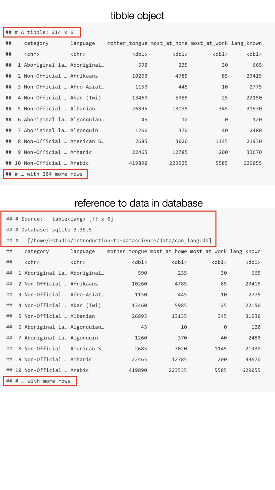
tbl(canlang_conn, "lang") in R with the show_query function from the dbplyr package.
show_query(tbl(canlang_conn, "lang"))
<SQL>
SELECT *
FROM `lang`
tbl(canlang_conn, "lang") in R, in the background, the function is translating the R code into SQL, sending that SQL to the database, and then translating the response for us. So dbplyr does all the hard work of translating from R to SQL and back for us; we can just stick with R!
lang_db table reference for the 2016 Canadian Census data in hand, we can mostly continue onward as if it were a regular data frame. For example, let’s do the same exercise from Chapter 1: we will obtain only those rows corresponding to Aboriginal languages, and keep only the language and mother_tongue columns. We can use the filter function to obtain only certain rows. Below we filter the data to include only Aboriginal languages.
aboriginal_lang_db <- filter(lang_db, category == "Aboriginal languages")
aboriginal_lang_db
## # Source:   SQL [?? x 6]
## # Database: sqlite 3.41.2 [/home/rstudio/introduction-to-datascience/data/can_lang.db]
##    category          language mother_tongue most_at_home most_at_work lang_known
##    <chr>             <chr>            <dbl>        <dbl>        <dbl>      <dbl>
##  1 Aboriginal langu… Aborigi…           590          235           30        665
##  2 Aboriginal langu… Algonqu…            45           10            0        120
##  3 Aboriginal langu… Algonqu…          1260          370           40       2480
##  4 Aboriginal langu… Athabas…            50           10            0         85
##  5 Aboriginal langu… Atikame…          6150         5465         1100       6645
##  6 Aboriginal langu… Babine …           110           20           10        210
##  7 Aboriginal langu… Beaver             190           50            0        340
##  8 Aboriginal langu… Blackfo…          2815         1110           85       5645
##  9 Aboriginal langu… Carrier           1025          250           15       2100
## 10 Aboriginal langu… Cayuga              45           10           10        125
## # ℹ more rows
SQL [?? x 6] and the output says ... more rows at the end (both indicating that R does not know how many rows there are in total!), and a database type sqlite is listed. We didn’t use the collect function because we are not ready to bring the data into R yet. We can still use the database to do some work to obtain only the small amount of data we want to work with locally in R. Let’s add the second part of our database query: selecting only the language and mother_tongue columns using the select function.
aboriginal_lang_selected_db <- select(aboriginal_lang_db, language, mother_tongue)
aboriginal_lang_selected_db
## # Source:   SQL [?? x 2]
## # Database: sqlite 3.41.2 [/home/rstudio/introduction-to-datascience/data/can_lang.db]
##    language                     mother_tongue
##    <chr>                                <dbl>
##  1 Aboriginal languages, n.o.s.           590
##  2 Algonquian languages, n.i.e.            45
##  3 Algonquin                             1260
##  4 Athabaskan languages, n.i.e.            50
##  5 Atikamekw                             6150
##  6 Babine (Wetsuwet'en)                   110
##  7 Beaver                                 190
##  8 Blackfoot                             2815
##  9 Carrier                               1025
## 10 Cayuga                                  45
## # ℹ more rows
select function. In order to actually retrieve this data in R as a data frame, we use the collect function. Below you will see that after running collect, R knows that the retrieved data has 67 rows, and there is no database listed any more.
aboriginal_lang_data <- collect(aboriginal_lang_selected_db)
aboriginal_lang_data
## # A tibble: 67 × 2
##    language                     mother_tongue
##    <chr>                                <dbl>
##  1 Aboriginal languages, n.o.s.           590
##  2 Algonquian languages, n.i.e.            45
##  3 Algonquin                             1260
##  4 Athabaskan languages, n.i.e.            50
##  5 Atikamekw                             6150
##  6 Babine (Wetsuwet'en)                   110
##  7 Beaver                                 190
##  8 Blackfoot                             2815
##  9 Carrier                               1025
## 10 Cayuga                                  45
## # ℹ 57 more rows
dbplyr provides many more functions (not just filter) that you can use to directly feed the database reference (lang_db) into downstream analysis functions (e.g., ggplot2 for data visualization). But dbplyr does not provide every function that we need for analysis; we do eventually need to call collect. For example, look what happens when we try to use nrow to count rows in a data frame:
nrow(aboriginal_lang_selected_db)
[1] NA
tail to preview the last six rows of a data frame:
tail(aboriginal_lang_selected_db)
Error: tail() is not supported by sql sources
tbl function. Thus, once you have finished your data wrangling of the tbl database reference object, it is advisable to bring it into R as a data frame using collect. But be very careful using collect: databases are often very big, and reading an entire table into R might take a long time to run or even possibly crash your machine. So make sure you use filter and select on the database table to reduce the data to a reasonable size before using collect to read it into R!
dbConnect function is listed below:
dbname: the name of the database (a single PostgreSQL instance can host more than one database)
host: the URL pointing to where the database is located
user: the username for accessing the database
password: the password for accessing the database
RPostgres package instead of RSQLite in the dbConnect function call. Below we demonstrate how to connect to a version of the can_mov_db database, which contains information about Canadian movies. Note that the host, user, and password below are not real; you will not actually be able to connect to a database using this information.
library(RPostgres)
canmov_conn <- dbConnect(RPostgres::Postgres(), dbname = "can_mov_db",
                        host = "fakeserver.stat.ubc.ca", port = 5432,
                        user = "user0001", password = "abc123")
dbListTables to find out what tables are in the can_mov_db database:
dbListTables(canmov_conn)
[1] "themes"            "medium"            "titles"            "title_aliases"
[5] "forms"             "episodes"          "names"             "names_occupations"
[9] "occupation"        "ratings"
"ratings" table to find the lowest rating that exists in the can_mov_db database:
ratings_db <- tbl(canmov_conn, "ratings")
ratings_db
# Source:   table<ratings> [?? x 3]
# Database: postgres [user0001@fakeserver.stat.ubc.ca:5432/can_mov_db]
   title              average_rating num_votes
   <chr>                    <dbl>     <int>
 1 The Grand Seduction       6.6       150
 2 Rhymes for Young Ghouls   6.3      1685
 3 Mommy                     7.5      1060
 4 Incendies                 6.1      1101
 5 Bon Cop, Bad Cop          7.0       894
 6 Goon                      5.5      1111
 7 Monsieur Lazhar           5.6       610
 8 What if                   5.3      1401
 9 The Barbarian Invations   5.8        99
10 Away from Her             6.9      2311
# … with more rows
average_rating column using select:
avg_rating_db <- select(ratings_db, average_rating)
avg_rating_db
# Source:   SQL [?? x 1]
# Database: postgres [user0001@fakeserver.stat.ubc.ca:5432/can_mov_db]
   average_rating
            <dbl>
 1            6.6
 2            6.3
 3            7.5
 4            6.1
 5            7.0
 6            5.5
 7            5.6
 8            5.3
 9            5.8
10            6.9
# … with more rows
min to find the minimum rating in that column:
min(avg_rating_db)
Error in min(avg_rating_db) : invalid 'type' (list) of argument
collect function to bring the data into R for further computation:
avg_rating_data <- collect(avg_rating_db)
min(avg_rating_data)
[1] 1
.csv, .tsv, or any of the other plain text or Excel formats. We had to open a connection to the database, then use dbplyr to translate tidyverse-like commands (filter, select etc.) into SQL commands that the database understands, and then finally collect the results. And not all tidyverse commands can currently be translated to work with databases. For example, we can compute a mean with a database but can’t easily compute a median. So you might be wondering: why should we use databases at all?
.csv file!? Chaos would ensue!
.csv file
write_csv function from the tidyverse package. The default arguments for this file are to use a comma (,) as the delimiter and include column names. Below we demonstrate creating a new version of the Canadian languages data set without the official languages category according to the Canadian 2016 Census, and then writing this to a .csv file:
no_official_lang_data <- filter(can_lang, category != "Official languages")
write_csv(no_official_lang_data, "data/no_official_languages.csv")
read_* functions from the tidyverse. But as time goes on, it is increasingly uncommon to find data (especially large amounts of data) in this format available for download from a URL. Instead, websites now often offer something known as an application programming interface (API), which provides a programmatic way to ask for subsets of a data set. This allows the website owner to control who has access to the data, what portion of the data they have access to, and how much data they can access. Typically, the website owner will give you a token or key (a secret string of characters somewhat like a password) that you have to provide when accessing the API.
rvest R package [21] and accessing the NASA “Astronomy Picture of the Day” API using the httr2 R package [17].
<span class="result-meta">
        <span class="result-price">$800</span>
        <span class="housing">
            1br -
        </span>
        <span class="result-hood"> (13768 108th Avenue)</span>
        <span class="result-tags">
            <span class="maptag" data-pid="6786042973">map</span>
        </span>
        <span class="banish icon icon-trash" role="button">
            <span class="screen-reader-text">hide this posting</span>
        </span>
    <span class="unbanish icon icon-trash red" role="button"></span>
    <ahref="#" class="restore-link">
        <span class="restore-narrow-text">restore</span>
        <span class="restore-wide-text">restore this posting</span>
    </a>
    <span class="result-price">$2285</span>
</span>
<span class="result-price">$800</span>
< and >, like <span>) and a closing tag (the same with a slash, like </span>). HTML source code generally stores its data between opening and closing tags like these. Tags are keywords that tell the web browser how to display or format the content. Above you can see that the information we want ($800) is stored between an opening and closing tag (<span> and </span>). In the opening tag, you can also see a very useful “class”: class="result-price". Since we want R to programmatically sort through all of the source code for the website to find apartment prices, maybe we can look for all the tags with the "result-price" class, and grab the information between the opening and closing tag. Indeed, take a look at another line of the source snippet above:
<span class="result-price">$2285</span>
"result-price" class. Wonderful! Now that we know what pattern we are looking for—a dollar amount between opening and closing tags that have the "result-price" class—we should be able to use code to pull out all of the matching patterns from the source code to obtain our data. This sort of “pattern” is known as a CSS selector (where CSS stands for cascading style sheet).
.result-price in its toolbar, and highlights all the other apartment prices that would be obtained using that selector (Figure 2.8.3).
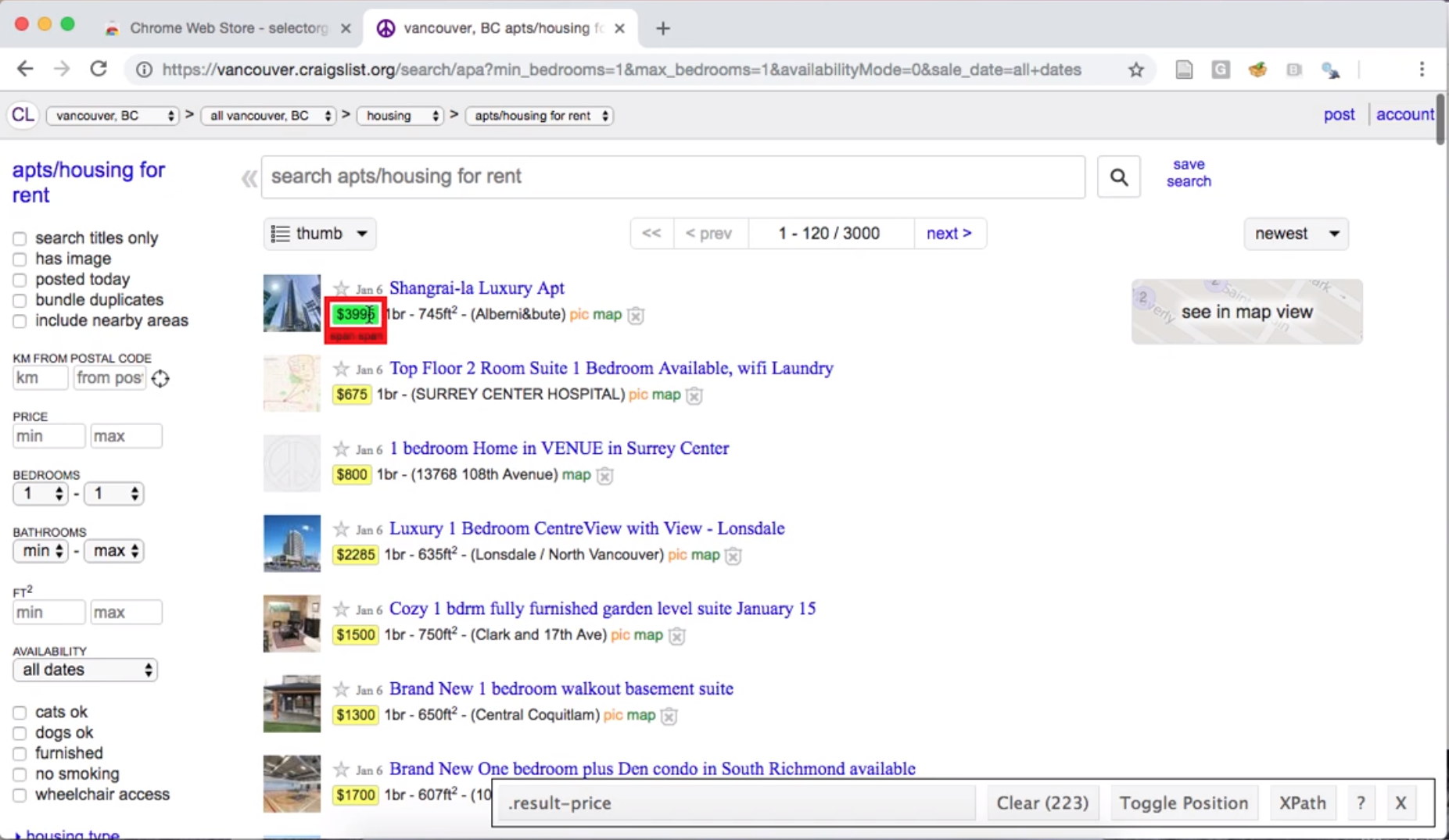
span selector, and highlights many of the lines on the page; this indicates that the span selector is not specific enough to capture only apartment sizes (Figure 2.8.4).
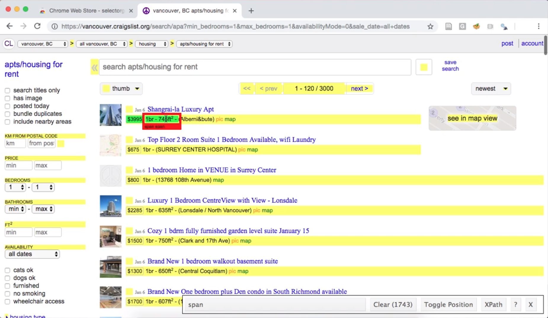
.housing selector (Figure 2.8.5).
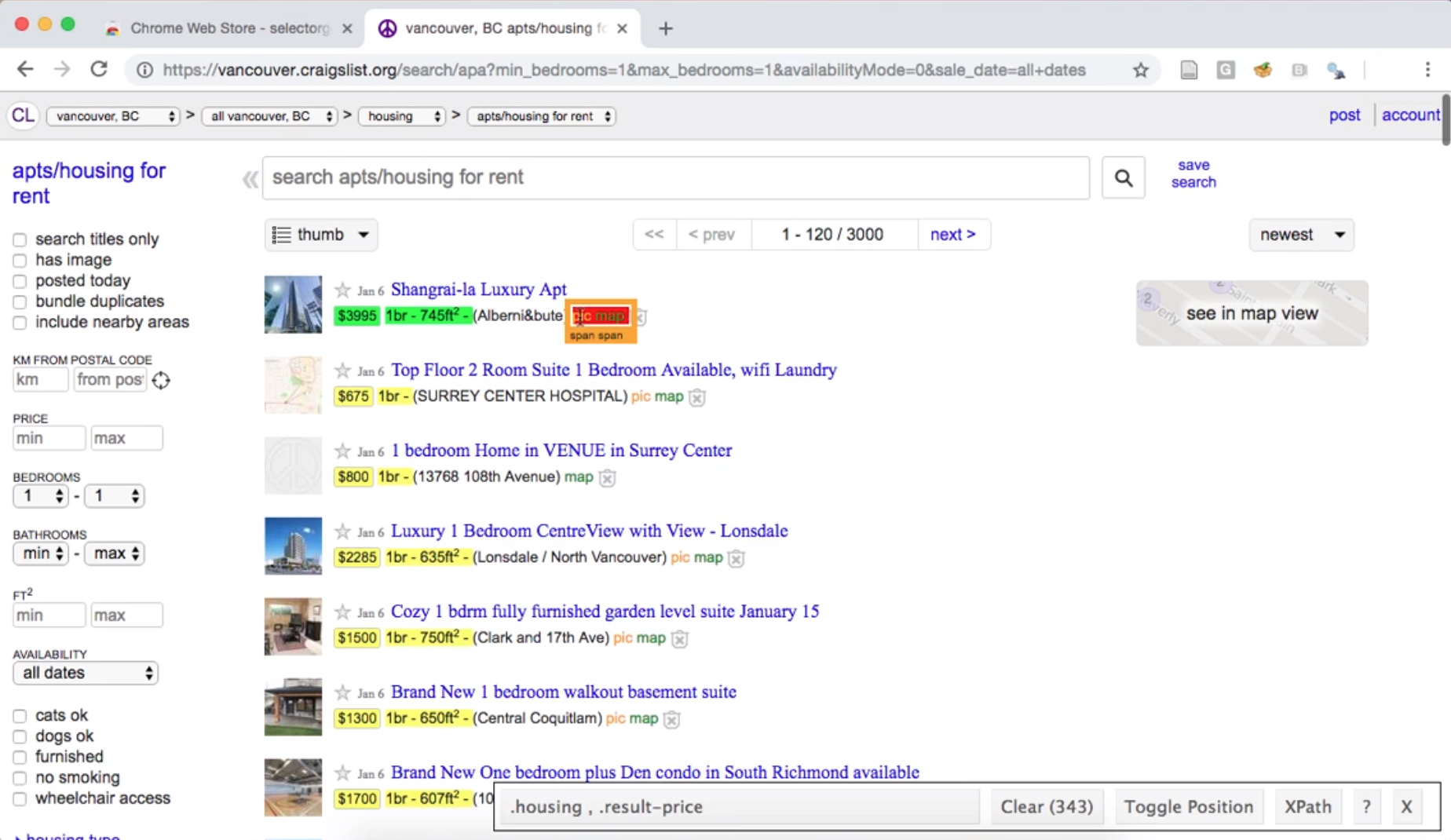
.housing and .result-price, respectively. The SelectorGadget returns them to us as a comma-separated list (here .housing , .result-price), which is exactly the format we need to provide to R if we are using more than one CSS selector.
robots.txt file and the Terms of Service document. If we take a look at Craigslist’s Terms of Service document, we find the following text: “You agree not to copy/collect CL content via robots, spiders, scripts, scrapers, crawlers, or any automated or manual equivalent (e.g., by hand).” So unfortunately, without explicit permission, we are not allowed to scrape the website.
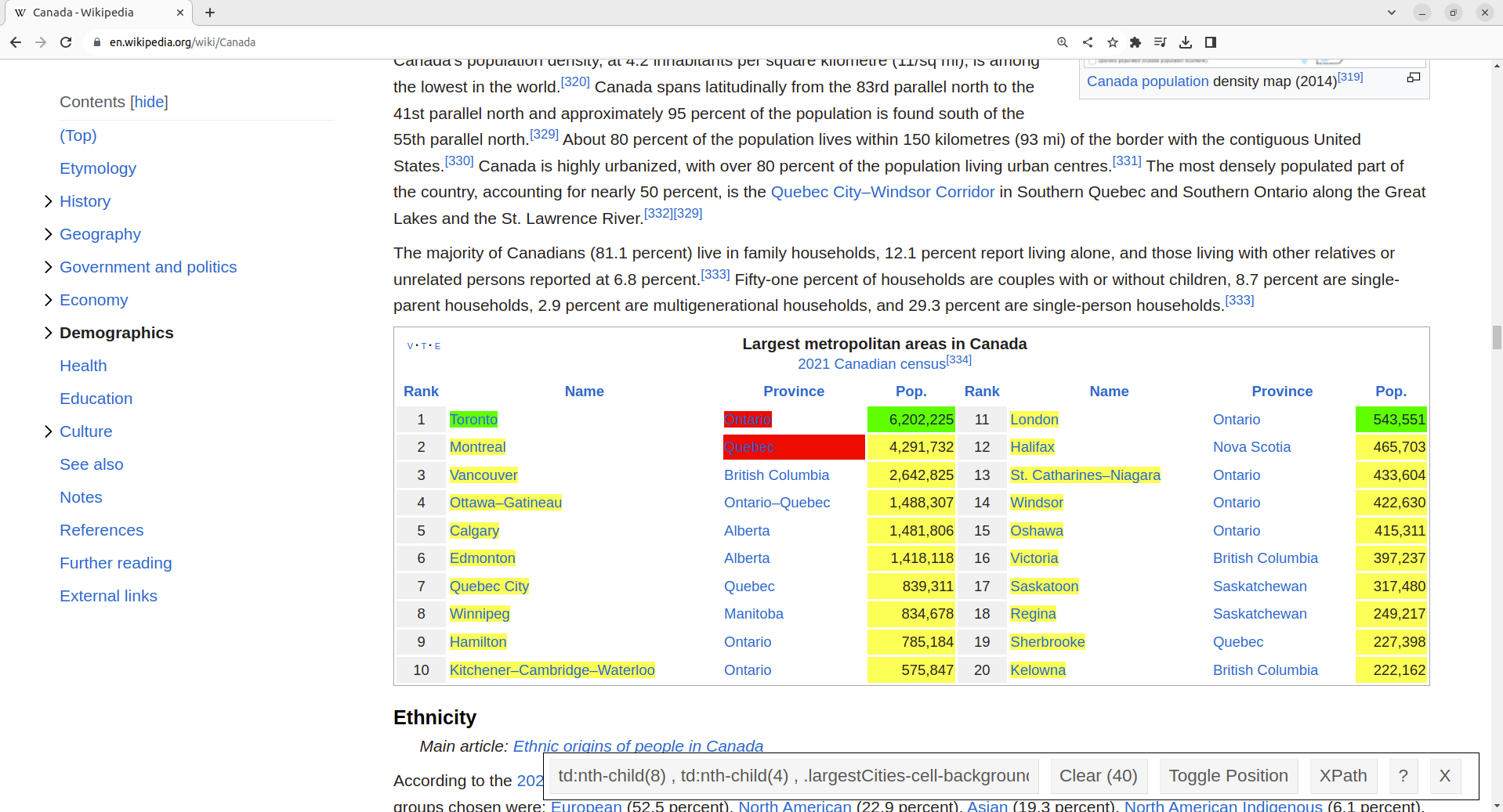
td:nth-child(8) ,
td:nth-child(4) ,
.largestCities-cell-background+ td a
rvest
rvest R package to scrape data from the Wikipedia page. We start by loading the rvest package:
library(rvest)
read_html:
page <- read_html("https://en.wikipedia.org/wiki/Canada")
read_html function directly downloads the source code for the page at the URL you specify, just like your browser would if you navigated to that site. But instead of displaying the website to you, the read_html function just returns the HTML source code itself, which we have stored in the page variable. Next, we send the page object to the html_nodes function, along with the CSS selectors we obtained from the SelectorGadget tool. Make sure to surround the selectors with quotation marks; the function html_nodes expects that argument is a string. We store the result of the html_nodes function in the population_nodes variable. Note that below we use the paste function with a comma separator (sep=",") to build the list of selectors. The paste function converts elements to characters and combines the values into a list. We use this function to build the list of selectors to maintain code readability; this avoids having a very long line of code.
selectors <- paste("td:nth-child(8)",
             "td:nth-child(4)",
             ".largestCities-cell-background+ td a", sep = ",")

population_nodes <- html_nodes(page, selectors)
head(population_nodes)
## {xml_nodeset (6)}
## [1] <a href="/wiki/Greater_Toronto_Area" title="Greater Toronto Area">Toronto ...
## [2] <td style="text-align:right;">6,202,225</td>
## [3] <a href="/wiki/London,_Ontario" title="London, Ontario">London</a>
## [4] <td style="text-align:right;">543,551\n</td>
## [5] <a href="/wiki/Greater_Montreal" title="Greater Montreal">Montreal</a>
## [6] <td style="text-align:right;">4,291,732</td>
head is a function that is often useful for viewing only a short summary of an R object, rather than the whole thing (which may be quite a lot to look at). For example, here head shows us only the first 6 items in the population_nodes object. Note that some R objects by default print only a small summary. For example, tibble data frames only show you the first 10 rows. But not all R objects do this, and that’s where the head function helps summarize things for you.
population_nodes list is a node from the HTML document that matches the CSS selectors you specified. A node is an HTML tag pair (e.g., <td> and </td>, which defines the cell of a table) combined with the content stored between the tags. For our CSS selector td:nth-child(4), an example node that that would be selected would be:
<td style="text-align:left;background:#f0f0f0;">
<a href="/wiki/London,_Ontario" title="London, Ontario">London</a>
</td>
html_text function. In the case of the example node above, html_text returns "London".
population_text <- html_text(population_nodes)
head(population_text)
## [1] "Toronto" "6,202,225" "London" "543,551\n" "Montreal" "4,291,732"
\n). In Chapter 3, we will learn more about how to wrangle data such as this into a more useful format for data analysis using R.
httr2 package in R to access data from the NASA “Astronomy Picture of the Day” API. Take a look at the stunning picture of the Rho-Ophiuchi cloud complex [19] in Figure 2.8.8 from July 13, 2023!

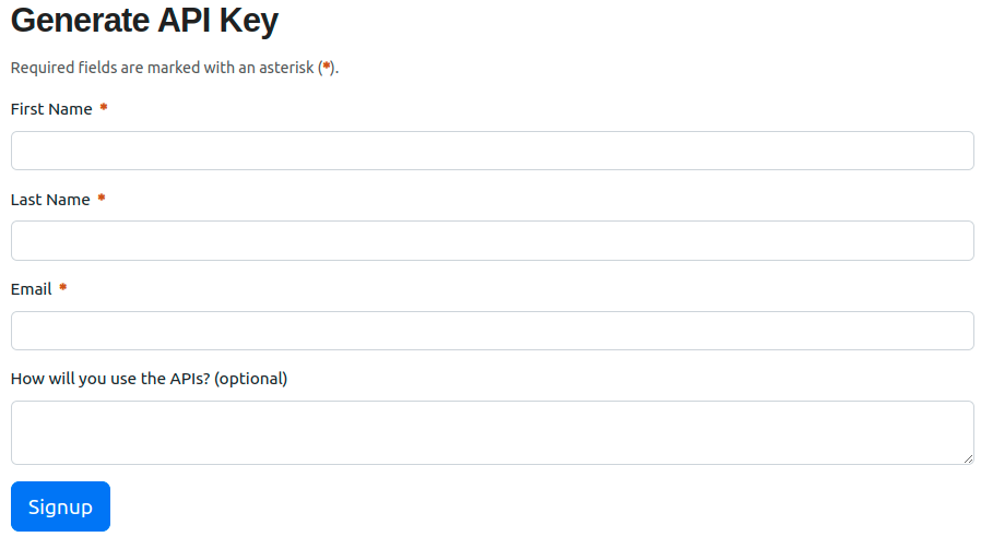
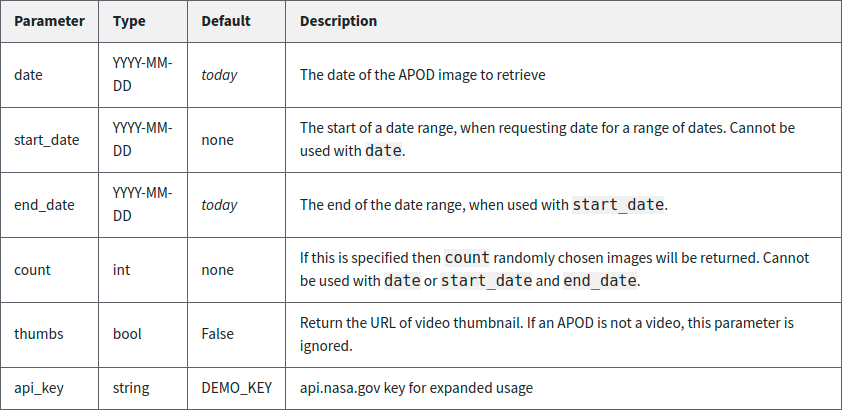
https://api.nasa.gov/planetary/apod. Second, we write ?, which denotes that a list of query parameters will follow. And finally, we specify a list of query parameters of the form parameter=value, separated by & characters. The NASA “Astronomy Picture of the Day” API accepts the parameters shown in Figure 2.8.11.
api_key=YOUR_API_KEY and date=2023-07-13. Remember to replace YOUR_API_KEY with the API key you received from NASA in your email! Putting it all together, the query will look like the following:
https://api.nasa.gov/planetary/apod?api_key=YOUR_API_KEY&date=2023-07-13
{"date":"2023-07-13","explanation":"A mere 390 light-years away, Sun-like stars
and future planetary systems are forming in the Rho Ophiuchi molecular cloud
complex, the closest star-forming region to our fair planet. The James Webb
Space Telescope's NIRCam peered into the nearby natal chaos to capture this
infrared image at an inspiring scale. The spectacular cosmic snapshot was
released to celebrate the successful first year of Webb's exploration of the
Universe. The frame spans less than a light-year across the Rho Ophiuchi region
and contains about 50 young stars. Brighter stars clearly sport Webb's
characteristic pattern of diffraction spikes. Huge jets of shocked molecular
hydrogen blasting from newborn stars are red in the image, with the large,
yellowish dusty cavity carved out by the energetic young star near its center.
Near some stars in the stunning image are shadows cast by their protoplanetary
disks.","hdurl":"https://apod.nasa.gov/apod/image/2307/STScI-01_RhoOph.png",
"media_type":"image","service_version":"v1","title":"Webb's
Rho Ophiuchi","url":"https://apod.nasa.gov/apod/image/2307/STScI-01_RhoOph1024.png"}
key : value pairs separated by commas. For example, if you look closely, you’ll see that the first entry is "date":"2023-07-13", which indicates that we indeed successfully received data corresponding to July 13, 2023.
httr2 package, and construct the query using the request function, which takes a single URL argument; you will recognize the same query URL that we pasted into the browser earlier. We will then send the query using the req_perform function, and finally obtain a JSON representation of the response using the resp_body_json function.
library(httr2)

req <- request("https://api.nasa.gov/planetary/apod?api_key=YOUR_API_KEY&date=2023-07-13")
resp <- req_perform(req)
nasa_data_single <- resp_body_json(resp)
nasa_data_single
## $date
## [1] "2023-07-13"
##
## $explanation
## [1] "A mere 390 light-years away, Sun-like stars and future planetary systems are forming in the Rho Ophiuchi molecular cloud complex, the closest star-forming region to our fair planet. The James Webb Space Telescope's NIRCam peered into the nearby natal chaos to capture this infrared image at an inspiring scale. The spectacular cosmic snapshot was released to celebrate the successful first year of Webb's exploration of the Universe. The frame spans less than a light-year across the Rho Ophiuchi region and contains about 50 young stars. Brighter stars clearly sport Webb's characteristic pattern of diffraction spikes. Huge jets of shocked molecular hydrogen blasting from newborn stars are red in the image, with the large, yellowish dusty cavity carved out by the energetic young star near its center. Near some stars in the stunning image are shadows cast by their protoplanetary disks."
##
## $hdurl
## [1] "https://apod.nasa.gov/apod/image/2307/STScI-01_RhoOph.png"
##
## $media_type
## [1] "image"
##
## $service_version
## [1] "v1"
##
## $title
## [1] "Webb's Rho Ophiuchi"
##
## $url
## [1] "https://apod.nasa.gov/apod/image/2307/STScI-01_RhoOph1024.png"
start_date and end_date parameters, as shown in the table of parameters in Figure 2.8.11. Let’s obtain all the records between May 1, 2023, and July 13, 2023; now the response will take the form of an R list (you’ll learn more about these in Chapter 3). Each item in the list will correspond to a single day’s record (just like the nasa_data_single object), and there will be 74 items total, one for each day between the start and end dates:
req <- request("https://api.nasa.gov/planetary/apod?api_key=YOUR_API_KEY&start_date=2023-05-01&end_date=2023-07-13")
resp <- req_perform(req)
nasa_data <- resp_body_json(resp)
length(nasa_data)
[1] 74
date, title, copyright, and url variables from the JSON data, and construct a data frame using the extracted information.
nasa_df_all <- tibble(bind_rows(lapply(nasa_data, as.data.frame.list)))
nasa_df <- select(nasa_df_all, date, title, copyright, url)
nasa_df
## # A tibble: 74 × 4
##    date       title                                        copyright       url
##    <chr>      <chr>                                        <chr>           <chr>
##  1 2023-05-01 Carina Nebula North                          "\nCarlos Tayl… http…
##  2 2023-05-02 Flat Rock Hills on Mars                      "\nNASA, \nJPL… http…
##  3 2023-05-03 Centaurus A: A Peculiar Island of Stars      "\nMarco Loren… http…
##  4 2023-05-04 The Galaxy, the Jet, and a Famous Black Hole  <NA>           http…
##  5 2023-05-05 Shackleton from ShadowCam                     <NA>           http…
##  6 2023-05-06 Twilight in a Flower                         "Dario Giannob… http…
##  7 2023-05-07 The Helix Nebula from CFHT                    <NA>           http…
##  8 2023-05-08 The Spanish Dancer Spiral Galaxy              <NA>           http…
##  9 2023-05-09 Shadows of Earth                             "\nMarcella Gi… http…
## 10 2023-05-10 Milky Way over Egyptian Desert               "\nAmr Abdulwa… http…
## # ℹ 64 more rows
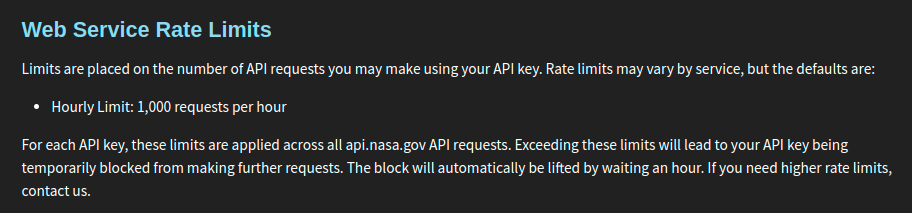
nasa_df data frame is stored on your machine, and you can play with it to your heart’s content. For example, you can use write_csv to save it to a file and read_csv to read it into R again later; and after reading the next few chapters you will have the skills to do even more interesting things! If you decide that you want to ask any of the various NASA APIs for more data (see the list of awesome NASA APIs here for more examples of what is possible), just be mindful as usual about how much data you are requesting and how frequently you are making requests.
readr documentation provides the documentation for many of the reading functions we cover in this chapter. It is where you should look if you want to learn more about the functions in this chapter, the full set of arguments you can use, and other related functions. The site also provides a very nice cheat sheet that summarizes many of the data wrangling functions from this chapter.
readxl documentation provides more details on reading data from Excel, such as reading in data with multiple sheets, or specifying the cells to read in.
rio R package [20] provides an alternative set of tools for reading and writing data in R. It aims to be a “Swiss army knife” for data reading/writing/converting, and supports a wide variety of data types (including data formats generated by other statistical software like SPSS and SAS).

