load(file.path(projecthome, "data","clinicaltrial.Rdata"))
xtabs( ~ drug + therapy, clin.trial )
##           therapy
## drug       no.therapy CBT
##   placebo           3   3
##   anxifree          3   3
##   joyzepam          3   3
mood.gain experienced by each person. In that chapter we did find a significant effect of drug, but at the end of the chapter we also ran an analysis to see if there was an effect of therapy. We didn’t find one, but there’s something a bit worrying about trying to run two separate analyses trying to predict the same outcome. Maybe there actually is an effect of therapy on mood gain, but we couldn’t find it because it was being "hidden" by the effect of drug? In other words, we’re going to want to run a single analysis that includes both drug and therapy as predictors. For this analysis each person is cross-classified by the drug they were given (a factor with 3 levels) and what therapy they received (a factor with 2 levels). We refer to this as a \(3 \times 2\) factorial design. If we cross-tabulate drug by therapy, using the xtabs() function (see Section 7.1), we get the following table:xtabs(~ drug+gender, clin.trial).
load(file.path(projecthome, "data","clinicaltrial.Rdata"))
xtabs( ~ drug + therapy, clin.trial )
## therapy ## drug no.therapy CBT ## placebo 3 3 ## anxifree 3 3 ## joyzepam 3 3
aggregate( mood.gain ~ drug + therapy, clin.trial, mean )
##       drug    therapy mood.gain
## 1  placebo no.therapy  0.300000
## 2 anxifree no.therapy  0.400000
## 3 joyzepam no.therapy  1.466667
## 4  placebo        CBT  0.600000
## 5 anxifree        CBT  1.033333
## 6 joyzepam        CBT  1.500000
aggregate( mood.gain ~ drug, clin.trial, mean )
aggregate( mood.gain ~ therapy, clin.trial, mean )
##       drug mood.gain
## 1  placebo 0.4500000
## 2 anxifree 0.7166667
## 3 joyzepam 1.4833333
mean( clin.trial$mood.gain )
## [1] 0.8833333
| no therapy | CBT | total | |
|---|---|---|---|
| placebo | 0.30 | 0.60 | 0.45 |
| anxifree | 0.40 | 1.03 | 0.72 |
| joyzepam | 1.47 | 1.50 | 1.48 |
| total | 0.72 | 1.04 | 0.88 |
drug), and each column corresponds to a different level of Factor B (in this case therapy). If we let \(R\) denote the number of rows in the table, and \(C\) denote the number of columns, we can refer to this as an \(R \times C\) factorial ANOVA. In this case \(R=3\) and \(C=2\text{.}\) We’ll use lowercase letters to refer to specific rows and columns, so \(\mu_{rc}\) refers to the population mean associated with the \(r\)th level of Factor A (i.e. row number \(r\)) and the \(c\)th level of Factor B (column number \(c\)).| no therapy | CBT | total | |
|---|---|---|---|
| placebo | \(\mu_{11}\) | \(\mu_{12}\) | |
| anxifree | \(\mu_{21}\) | \(\mu_{22}\) | |
| joyzepam | \(\mu_{31}\) | \(\mu_{32}\) | |
| total |
| no therapy | CBT | total | |
|---|---|---|---|
| placebo | \(\mu_{11}\) | \(\mu_{12}\) | \(\mu_{1.}\) |
| anxifree | \(\mu_{21}\) | \(\mu_{22}\) | \(\mu_{2.}\) |
| joyzepam | \(\mu_{31}\) | \(\mu_{32}\) | \(\mu_{3.}\) |
| total | \(\mu_{.1}\) | \(\mu_{.2}\) | \(\mu_{..}\) |
drug) to predict our outcome variable (i.e., mood.gain), and so this was what we did:
model.1 <- aov( mood.gain ~ drug, clin.trial )
summary( model.1 )
##             Df Sum Sq Mean Sq F value   Pr(>F)
## drug         2  3.453  1.7267   18.61 8.65e-05 ***
## Residuals   15  1.392  0.0928
## ---
## Signif. codes:  0 '***' 0.001 '**' 0.01 '*' 0.05 '.' 0.1 ' ' 1
model.1 as the label for my aov object, since I’m planning on creating quite a few other models too. To start with, suppose I’m also curious to find out if therapy has a relationship to mood.gain. In light of what we’ve seen from our discussion of multiple regression in Chapter 15, you probably won’t be surprised that all we have to do is extend the formula: in other words, if we specify mood.gain ~ drug + therapy as our model, we’ll probably get what we’re after:
model.2 <- aov( mood.gain ~ drug + therapy, clin.trial )
summary( model.2 )
##             Df Sum Sq Mean Sq F value   Pr(>F)
## drug         2  3.453  1.7267   18.61 8.65e-05 ***
## therapy      1   0.47   0.467    7.08    0.019 *
## Residuals   14   0.92   0.066
## ---
## Signif. codes:  0 '***' 0.001 '**' 0.01 '*' 0.05 '.' 0.1 ' ' 1
drug factor, along with a corresponding between-group \(df\) value. It also calculates a mean square value (MS), and \(F\)-statistic and a \(p\)-value. There is also a row corresponding to the therapy factor, and a row corresponding to the residuals (i.e., the within groups variation).
drug, therapy or the residuals. To see this, let’s not worry about how the sums of squares values are calculated: instead, let’s take it on faith that R has calculated the SS values correctly, and try to verify that all the rest of the numbers make sense. First, note that for the drug factor, we divide \(3.45\) by \(2\text{,}\) and end up with a mean square value of \(1.73\text{.}\) For the therapy factor, there’s only 1 degree of freedom, so our calculations are even simpler: dividing \(0.47\) (the SS value) by 1 gives us an answer of \(0.47\) (the MS value).
drug factor and the other corresponding to the therapy factor. Regardless of which one we’re talking about, the \(F\) statistic is calculated by dividing the mean square value associated with the factor by the mean square value associated with the residuals. If we use "A" as shorthand notation to refer to the first factor (factor A; in this case drug) and "R" as shorthand notation to refer to the residuals, then the \(F\) statistic associated with factor A is denoted \(F_A\text{,}\) and is calculated as follows:
therapy). Note that this use of "R" to refer to residuals is a bit awkward, since we also used the letter R to refer to the number of rows in the table, but I’m only going to use "R" to mean residuals in the context of SS\(_R\) and MS\(_R\text{,}\) so hopefully this shouldn’t be confusing. Anyway, to apply this formula to the drugs factor, we take the mean square of \(1.73\) and divide it by the residual mean square value of \(0.07\text{,}\) which gives us an \(F\)-statistic of \(26.15\text{.}\) The corresponding calculation for the therapy variable would be to divide \(0.47\) by \(0.07\) which gives \(7.08\) as the \(F\)-statistic. Not surprisingly, of course, these are the same values that R has reported in the ANOVA table above.
drug factor we’re talking about an \(F\) distribution with 2 and 14 degrees of freedom (I’ll discuss degrees of freedom in more detail later). In contrast, for the therapy factor sampling distribution is \(F\) with 1 and 14 degrees of freedom. If we really wanted to, we could calculate the \(p\) value ourselves using the pf() function (see Section 9.6). Just to prove that there’s nothing funny going on, here’s what that would look like for the drug variable:
pf( q=26.15, df1=2, df2=14, lower.tail=FALSE )
## [1] 1.871981e-05
model.2 should be read in much the same way as the ANOVA table for the simpler analysis for model.1. In short, it’s telling us that the factorial ANOVA for our \(3 \times 2\) design found a significant effect of drug (\(F_{2,14} = 26.15, p < .001\)) as well as a significant effect of therapy (\(F_{1,14} = 7.08, p = .02\)). Or, to use the more technically correct terminology, we would say that there are two main effects of drug and therapy. At the moment, it probably seems a bit redundant to refer to these as "main" effects: but it actually does make sense. Later on, we’re going to want to talk about the possibility of "interactions" between the two factors, and so we generally make a distinction between main effects and interaction effects.
formula argument to the aov() function. Secondly, I wanted to show you what the ANOVA table looks like in this case, so that you can see from the outset that the basic logic and structure behind factorial ANOVA is the same as that which underpins one way ANOVA. Try to hold onto that feeling. It’s genuinely true, insofar as factorial ANOVA is built in more or less the same way as the simpler one-way ANOVA model. It’s just that this feeling of familiarity starts to evaporate once you start digging into the details. Traditionally, this comforting sensation is replaced by an urge to murder the the authors of statistics textbooks.
| no therapy | CBT | total | |
|---|---|---|---|
| placebo | \(\bar{Y}_{11}\) | \(\bar{Y}_{12}\) | \(\bar{Y}_{1.}\) |
| anxifree | \(\bar{Y}_{21}\) | \(\bar{Y}_{22}\) | \(\bar{Y}_{2.}\) |
| joyzepam | \(\bar{Y}_{31}\) | \(\bar{Y}_{32}\) | \(\bar{Y}_{3.}\) |
| total | \(\bar{Y}_{.1}\) | \(\bar{Y}_{.2}\) | \(\bar{Y}_{..}\) |
drugs factor has 3 levels and the therapy factor has 2 levels, and so what we’re trying to run is a \(3 \times 2\) factorial ANOVA. However, we’ll be a little more general and say that Factor A (the row factor) has \(R\) levels and Factor B (the column factor) has \(C\) levels, and so what we’re runnning here is an \(R \times C\) factorial ANOVA.
anxifree drug: one for people with no.therapy, and one for the CBT group. Not only that, within each of these cells there are \(N\) observations. So, if we want to convert our SS value into a quantity that calculates the between-groups sum of squares on a "per observation" basis, we have to multiply by by \(N \times C\text{.}\) The formula for factor B is of course the same thing, just with some subscripts shuffled around:
aggregate(), and we also calculated the grand mean. Let’s repeat those calculations, but this time we’ll save the results to varibles so that we can use them in subsequent calculations:
drug.means <- aggregate( mood.gain ~ drug, clin.trial, mean )[,2]
therapy.means <- aggregate( mood.gain ~ therapy, clin.trial, mean )[,2]
grand.mean <- mean( clin.trial$mood.gain )
drug. There are a total of \(N=3\) people in each group, and \(C=2\) different types of therapy. Or, to put it another way, there are \(3 \times 2 = 6\) people who received any particular drug. So our calculations are:
SS.drug <- (3*2) * sum( (drug.means - grand.mean)^2 )
SS.drug
## [1] 3.453333
SS.therapy <- (3*3) * sum( (therapy.means - grand.mean)^2 )
SS.therapy
## [1] 0.4672222
SS.tot <- sum( (clin.trial$mood.gain - grand.mean)^2 )
SS.tot
## [1] 4.845
SS.res <- SS.tot - (SS.drug + SS.therapy)
SS.res
## [1] 0.9244444
drugs factor we obtain \(df = 2\text{,}\) and for the therapy factor we obtain \(df=1\text{.}\) Later on on, when we discuss the interpretation of ANOVA as a regression model (see Section 16.6) I’ll give a clearer statement of how we arrive at this number, but for the moment we can use the simple definition of degrees of freedom, namely that the degrees of freedom equals the number of quantities that are observed, minus the number of constraints. So, for the drugs factor, we observe 3 separate group means, but these are constrained by 1 grand mean; and therefore the degrees of freedom is 2. For the residuals, the logic is similar, but not quite the same. The total number of observations in our experiment is 18. The constraints correspond to the 1 grand mean, the 2 additional group means that the drug factor introduces, and the 1 additional group mean that the the therapy factor introduces, and so our degrees of freedom is 14. As a formula, this is \(N-1 -(R-1)-(C-1)\text{,}\) which simplifies to \(N-R-C+1\text{.}\)
drug and 0.92 for therapy), as are the degrees of freedom (2 for drug, 1 for therapy). But they don’t give the same answers! Most notably, when we ran the one-way ANOVA for therapy in Section 14.11 we didn’t find a significant effect (the \(p\)-value was 0.21). However, when we look at the main effect of therapy within the context of the two-way ANOVA, we do get a significant effect (\(p=.019\)). The two analyses are clearly not the same.
therapy, and therefore ignore the effect of drug, the ANOVA will end up dumping all of the drug-induced variability into the residuals! This has the effect of making the data look more noisy than they really are, and the effect of therapy which is correctly found to be significant in the two-way ANOVA now becomes non-significant. If we ignore something that actually matters (e.g., drug) when trying to assess the contribution of something else (e.g., therapy) then our analysis will be distorted. Of course, it’s perfectly okay to ignore variables that are genuinely irrelevant to the phenomenon of interest: if we had recorded the colour of the walls, and that turned out to be non-significant in a three-way ANOVA (i.e. mood.gain ~ drug + therapy + wall.colour), it would be perfectly okay to disregard it and just report the simpler two-way ANOVA that doesn’t include this irrelevant factor. What you shouldn’t do is drop variables that actually make a difference!
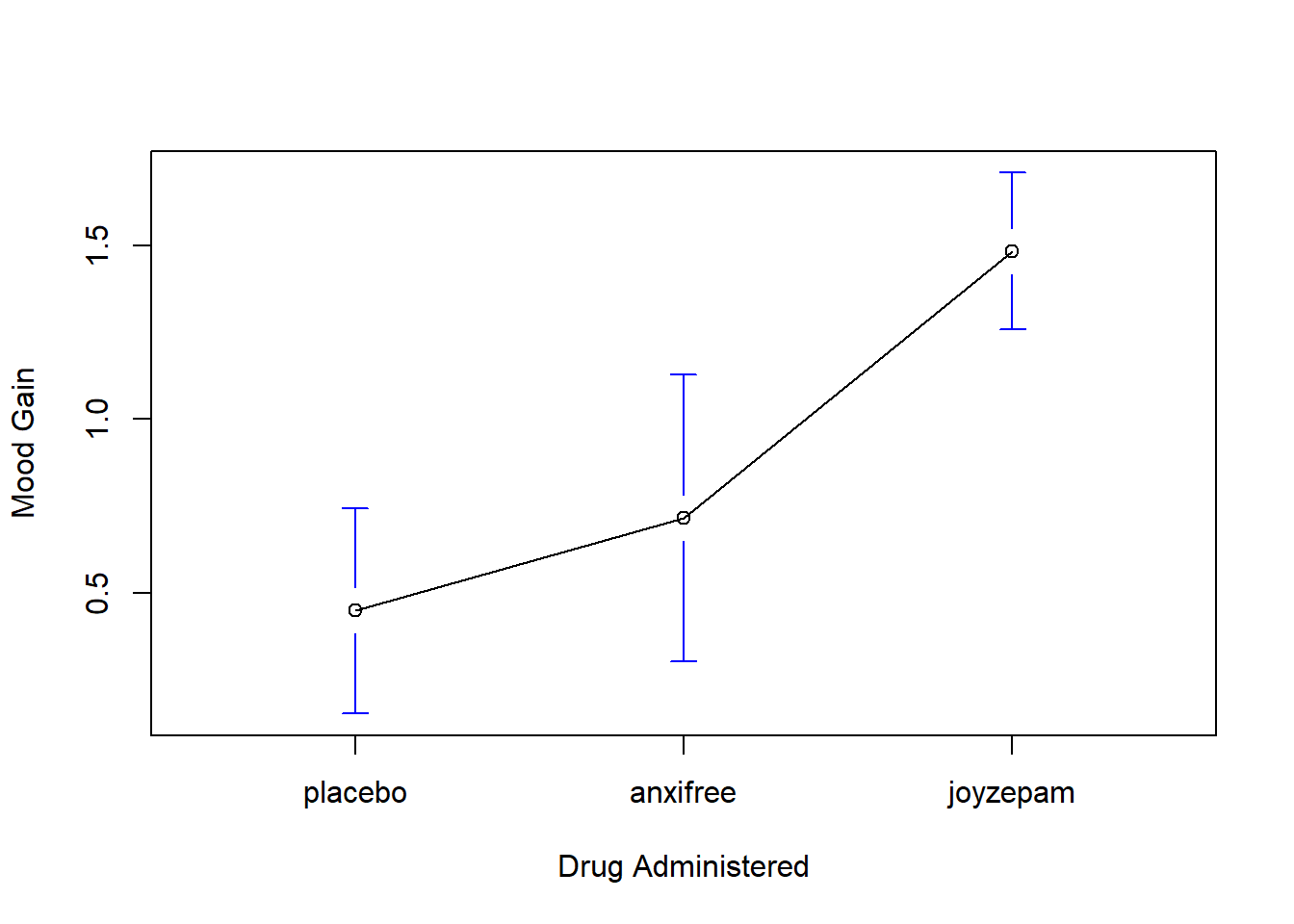
interaction.plot() function, but this function won’t draw error bars for you. A fairly simple function that will include error bars for you is the lineplot.CI() function in the sciplots package (see Subsection 10.5.4). The command
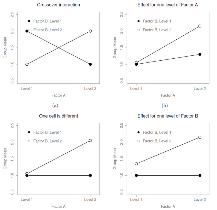
library(sciplot)
library(lsr)
 lineplot.CI( x.factor = clin.trial$drug,
              response = clin.trial$mood.gain,
              group = clin.trial$therapy,
              ci.fun = ciMean,
              xlab = "drug",
              ylab = "mood gain" )
ciMean function is in the lsr package, so you need to have lsr loaded!). Our main concern relates to the fact that the two lines aren’t parallel. The effect of CBT (difference between solid line and dotted line) when the drug is Joyzepam (right side) appears to be near zero, even smaller than the effect of CBT when a placebo is used (left side). However, when Anxifree is administered, the effect of CBT is larger than the placebo (middle). Is this effect real, or is this just random variation due to chance? Our original ANOVA cannot answer this question, because we make no allowances for the idea that interactions even exist! In this section, we’ll fix this problem.
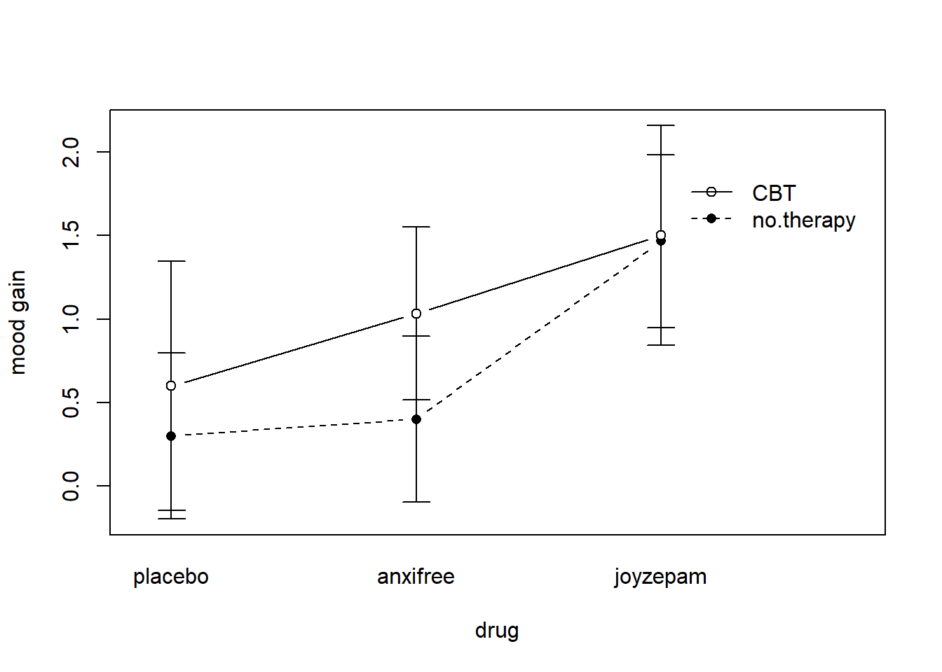
mood.gain ~ drug + therapy + drug:therapy so although there are only two factors involved in our model (i.e., drug and therapy), there are three distinct terms (i.e., drug, therapy and drug:therapy). That is, in addition to the main effects of drug and therapy, we have a new component to the model, which is our interaction term drug:therapy. Intuitively, the idea behind an interaction effect is fairly simple: it just means that the effect of Factor A is different, depending on which level of Factor B we’re talking about. But what does that actually mean in terms of our data? Figure 16.18 depicts several different patterns that, although quite different to each other, would all count as an interaction effect. So it’s not entirely straightforward to translate this qualitative idea into something mathematical that a statistician can work with. As a consequence, the way that the idea of an interaction effect is formalised in terms of null and alternative hypotheses is slightly difficult, and I’m guessing that a lot of readers of this book probably won’t be all that interested. Even so, I’ll try to give the basic idea here.
drug in our running example). We originally formulated this in terms of the null hypothesis that the two marginal means \(\mu_{r.}\) are all equal to each other. Obviously, if all of these are equal to each other, then they must also be equal to the grand mean \(\mu_{..}\) as well, right? So what we can do is define the effect of Factor A at level \(r\) to be equal to the difference between the marginal mean \(\mu_{r.}\) and the grand mean \(\mu_{..}\text{.}\) Let’s denote this effect by \(\alpha_r\text{,}\) and note that
drug and therapy, we include the interaction term drug:therapy. So the R command to create the ANOVA model now looks like this:
model.3 <- aov( mood.gain ~ drug + therapy + drug:therapy, clin.trial )
drug*therapy. The * operator inside the formula is taken to indicate that you want both main effects and the interaction. So we can also run our ANOVA like this, and get the same answer:
model.3 <- aov( mood.gain ~ drug * therapy, clin.trial )
summary( model.3 )
##              Df Sum Sq Mean Sq F value   Pr(>F)
## drug          2  3.453  1.7267  31.714 1.62e-05 ***
## therapy       1  0.467  0.4672   8.582   0.0126 *
## drug:therapy  2  0.271  0.1356   2.490   0.1246
## Residuals    12  0.653  0.0544
## ---
## Signif. codes:  0 '***' 0.001 '**' 0.01 '*' 0.05 '.' 0.1 ' ' 1
drug, it doesn’t tell you anything about which drugs are different to one another. To find that out, you need to run additional analyses. We’ll talk about some analyses that you can run in Section 16.7 and Section 16.8. The same is true for interaction effects: knowing that there’s a significant interaction doesn’t tell you anything about what kind of interaction exists. Again, you’ll need to run additional analyses.
etaSquared() function from the lsr package. As before, we input the aov object for which we want the \(\eta^2\) calculations performed, and R outputs a matrix showing the effect sizes for each term in the model. First, let’s have a look at the effect sizes for the original ANOVA without the interaction term:
etaSquared( model.2 )
##            eta.sq eta.sq.part
## drug    0.7127623   0.7888325
## therapy 0.0964339   0.3357285
drug accounts for 71.3% of the variance (i.e. \(\eta^2 = 0.713\)) in mood.gain, whereas therapy only accounts for 9.6%. This leaves a total of 19.1% of the variation unaccounted for (i.e., the residuals constitute 19.1% of the variation in the outcome). Overall, this implies that we have a very large effectdrug and a modest effect of therapy.
therapy isn’t all that large, controlling for it doesn’t make much of a difference, so the partial \(\eta^2\) for drug doesn’t increase very much, and we obtain a value of \(_p\eta^2 = 0.789\)). In contrast, because the effect of drug was very large, controlling for it makes a big difference, and so when we calculate the partial \(\eta^2\) for therapy you can see that it rises to \(_p\eta^2 = 0.336\text{.}\) The question that we have to ask ourselves is, what does these partial \(\eta^2\) values actually mean? The way I generally interpret the partial \(\eta^2\) for the main effect of Factor A is to interpret it as a statement about a hypothetical experiment in which only Factor A was being varied. So, even though in this experiment we varied both A and B, we can easily imagine an experiment in which only Factor A was varied: the partial \(\eta^2\) statistic tells you how much of the variance in the outcome variable you would expect to see accounted for in that experiment. However, it should be noted that this interpretation -- like many things associated with main effects -- doesn’t make a lot of sense when there is a large and significant interaction effect.
etaSquared( model.3 )
##                  eta.sq eta.sq.part
## drug         0.71276230   0.8409091
## therapy      0.09643390   0.4169559
## drug:therapy 0.05595689   0.2932692
effect() function in the effects package to do this (don’t forget to install the package if you don’t have it already!). If the ANOVA that you have run is a saturated model (i.e., contains all possible main effects and all possible interaction effects) then the estimates of the group means are actually identical to the sample means, though the confidence intervals will use a pooled estimate of the standard errors, rather than use a separate one for each group. To illustrate this, let’s apply the effect() function to our saturated model (i.e., model.3) for the clinical trial data. The effect() function contains two arguments we care about: the term argument specifies what terms in the model we want the means to be calculated for, and the mod argument specifies the model:
library(effects)
eff <- effect( term = "drug*therapy", mod = model.3 )
eff
##
##  drug*therapy effect
##           therapy
## drug       no.therapy      CBT
##   placebo    0.300000 0.600000
##   anxifree   0.400000 1.033333
##   joyzepam   1.466667 1.500000
group.means variable that we computed using aggregate()). One useful thing that we can do using the effect variable eff, however, is extract the confidence intervals using the summary() function:
summary(eff)
##
##  drug*therapy effect
##           therapy
## drug       no.therapy      CBT
##   placebo    0.300000 0.600000
##   anxifree   0.400000 1.033333
##   joyzepam   1.466667 1.500000
##
##  Lower 95 Percent Confidence Limits
##           therapy
## drug        no.therapy       CBT
##   placebo  0.006481093 0.3064811
##   anxifree 0.106481093 0.7398144
##   joyzepam 1.173147759 1.2064811
##
##  Upper 95 Percent Confidence Limits
##           therapy
## drug       no.therapy       CBT
##   placebo   0.5935189 0.8935189
##   anxifree  0.6935189 1.3268522
##   joyzepam  1.7601856 1.7935189
effect() function will calculate the value of the group means that would be expected on the basis of the marginal means (i.e., assuming no interaction). Using the notation we developed earlier, the estimate reported for \(\mu_{rc}\text{,}\) the mean for level \(r\) on the (row) Factor A and level \(c\) on the (column) Factor B would be \(\mu_{..} + \alpha_r + \beta_c\text{.}\) If there are genuinely no interactions between the two factors, this is actually a better estimate of the population mean than the raw sample mean would be. The command to obtain these estimates is actually identical to the last one, except that we use model.2. When you do this, R will give you a warning message:
eff <- effect( "drug*therapy", model.2 )
Warning message:
In analyze.model(term, mod, xlevels, default.levels) :
  drug:therapy does not appear in the model
"drug*therapy" as our input, we’re telling R that we want it to output the estimated group means (rather than marginal means), but the actual input "drug*therapy" might mean that you want interactions included or you might not. There’s no actual ambiguity here, because the model itself either does or doesn’t have interactions, but the authors of the function thought it sensible to include a warning just to make sure that you’ve specified the actual model you care about. But, assuming that we genuinely don’t believe that there are any interactions, model.2 is the right model to use, so we can ignore this warning.Effect() within the effects package that has slightly different arguments, but computes the same things, and won’t give you this warning message.
eff
##
##  drug*therapy effect
##           therapy
## drug       no.therapy       CBT
##   placebo   0.2888889 0.6111111
##   anxifree  0.5555556 0.8777778
##   joyzepam  1.3222222 1.6444444
summary( eff )
leveneTest() function in the car package to do this. This function expects that you have a saturated model (i.e., included all of the relevant terms), because the test is primarily concerned with the within-group variance, and it doesn’t really make a lot of sense to calculate this any way other than with respect to the full model. So we try either of the following commands:
leveneTest( model.2 )
leveneTest( mood.gain ~ drug + therapy, clin.trial )
## Error in leveneTest.formula(formula(y), data = model.frame(y), ...) :
##   Model must be completely crossed formula only.
leveneTest() function is implemented, however, if you use a formula like mood.gain ~ drug + therapy + drug:therapy, or input an ANOVA object based on a formula like this, you actually get the error message. That shouldn’t happen, because this actually is a fully crossed model. However, there’s a quirky shortcut in the way that the leveneTest() function checks whether your model is fully crossed that means that it doesn’t recognise this as a fully crossed model. Essentially what the function is doing is checking that you used * (which ensures that the model is fully crossed), and not + or : in your model formula. So if you’ve manually typed out all of the relevant terms for a fully crossed model, the leveneTest() function doesn’t detect it. I think this is a bug.
library(car)
 leveneTest( model.3 )
 leveneTest( mood.gain ~ drug * therapy, clin.trial )
## Levene's Test for Homogeneity of Variance (center = median)
##       Df F value Pr(>F)
## group  5  0.0955 0.9912
##       12
residuals() function to extract the residuals from the model itself, and then we can examine those residuals in a few different ways. It’s generally a good idea to examine them graphically, by drawing histograms (i.e., hist() function) and QQ plots (i.e., qqnorm() function. If you want a formal test for the normality of the residuals, then we can run the Shapiro-Wilk test (i.e., shapiro.test()). If we wanted to check the residuals with respect to model.2 (i.e., the model with both main effects but no interactions) then we could do the following:
resid <- residuals( model.2 )  # pull the residuals
hist( resid )                  # draw a histogram
qqnorm( resid )                # draw a normal QQ plot
shapiro.test( resid )          # run the Shapiro-Wilk test
##
##  Shapiro-Wilk normality test
##
## data:  resid
## W = 0.95635, p-value = 0.5329
therapy. I’m not fussy: I don’t care if it’s a main effect or an interaction effect.model.3 earlier: in this model we did see a main effect of therapy (\(p=.013\)) but we did not see an interaction effect (\(p=.125\)). That’s kind of telling us what we want to know, but it’s not quite the same thing. What we really want is a single test that jointly checks the main effect of therapy and the interaction effect.
model.3, and it contains a main effect for therapy, a main effect for drug, and the drug by therapy interaction term. The null model would be model.1 since it contains only the main effect of drug.
Y ~ A + B + C + D. Our null model only contains some subset of these terms, say Y ~ A + B. Some of these terms might be main effect terms, others might be interaction terms. It really doesn’t matter. The only thing that matters here is that we want to treat some of these terms as the "starting point" (i.e. the terms in the null model, A and B), and we want to see if including the other terms (i.e., C and D) leads to a significant improvement in model performance, over and above what could be achieved by a model that includes only A and B. In essence, we have null and alternative hypotheses that look like this:
| Hypothesis | Correct model? | R formula for correct model |
|---|---|---|
| Null | \(M0\) | Y ~ A + B |
| Alternative | \(M1\) | Y ~ A + B + C + D |
model.1, which stipulates that there is a main effect of drug, but no other effects exist. We expressed this via the model formula mood.gain ~ drug. The alternative model here is model.3, which stipulates that there is a main effect of drug, a main effect of therapy, and an interaction. If we express this in the "long" format, this model corresponds to the formula mood.gain ~ drug + therapy + drug:therapy, though we often express this using the * shorthand. The key thing here is that if we compare model.1 to model.3, we’re lumping the main effect of therapy and the interaction term together. Running this test in R is straightforward: we just input both models to the anova() function, and it will run the exact \(F\)-test that I outlined above.
anova( model.1, model.3 )
## Analysis of Variance Table
##
## Model 1: mood.gain ~ drug
## Model 2: mood.gain ~ drug * therapy
##   Res.Df     RSS Df Sum of Sq      F  Pr(>F)
## 1     15 1.39167
## 2     12 0.65333  3   0.73833 4.5204 0.02424 *
## ---
## Signif. codes:  0 '***' 0.001 '**' 0.01 '*' 0.05 '.' 0.1 ' ' 1
model.1 and model.3 you can reassure yourself that the RSS values printed in this table really do correspond to the residual sum of squares associated with these two models. So let’s type them in as variables:
ss.res.null <- 1.392
ss.res.full <- 0.653
ss.diff <- ss.res.null - ss.res.full
ss.diff
## [1] 0.739
model.3: it’s the total sample size \(N\text{,}\) minus the total number of groups \(G\) that are relevant to the model. We have 18 people in the trial and 6 possible groups (i.e., 2 therapies \(\times\) 3 drugs), so the degrees of freedom here is 12. The degrees of freedom for the null model are calculated similarly. The only difference here is that there are only 3 relevant groups (i.e., 3 drugs), so the degrees of freedom here is 15. And, because the degrees of freedom associated with the difference is equal to the difference in the two degrees of freedom, we arrive at the conclusion that we have \(15-12 = 3\) degrees of freedom. Now that we know the degrees of freedom, we can calculate our MS values:
ms.res <- ss.res.full / 12
ms.diff <- ss.diff / 3
F.stat <- ms.diff / ms.res
F.stat
## [1] 4.526799
anova() function produced earlier.
lm() is kind of a hint too. When we use an R formula like outcome ~ predictor1 + predictor2 what we’re really working with is the somewhat uglier linear model:
grade that a student receives in my class, a ratio-scale variable corresponding to a mark from 0% to 100%. There are two predictor variables of interest: whether or not the student turned up to lectures (the attend variable), and whether or not the student actually read the textbook (the reading variable). We’ll say that attend = 1 if the student attended class, and attend = 0 if they did not. Similarly, we’ll say that reading = 1 if the student read the textbook, and reading = 0 if they did not.
grade of the \(p\)-th student in the class. This is not quite the same notation that we used earlier in this chapter: previously, we’ve used the notation \(Y_{rci}\) to refer to the \(i\)-th person in the \(r\)-th group for predictor 1 (the row factor) and the \(c\)-th group for predictor 2 (the column factor). This extended notation was really handy for describing how the SS values are calculated, but it’s a pain in the current context, so I’ll switch notation here. Now, the \(Y_p\) notation is visually simpler than \(Y_{rci}\text{,}\) but it has the shortcoming that it doesn’t actually keep track of the group memberships! That is, if I told you that \(Y_{0,0,3} = 35\text{,}\) you’d immediately know that we’re talking about a student (the 3rd such student, in fact) who didn’t attend the lectures (i.e., attend = 0) and didn’t read the textbook (i.e. reading = 0), and who ended up failing the class (grade = 35). But if I tell you that \(Y_p = 35\) all you know is that the \(p\)-th student didn’t get a good grade. We’ve lost some key information here. Of course, it doesn’t take a lot of thought to figure out how to fix this: what we’ll do instead is introduce two new variables \(X_{1p}\) and \(X_{2p}\) that keep track of this information. In the case of our hypothetical student, we know that \(X_{1p} = 0\) (i.e., attend = 0) and \(X_{2p} = 0\) (i.e., reading = 0). So the data might look like this:
| person \(p\) | grade \(Y_p\) | attendance \(X_{1p}\) | reading \(X_{2p}\) |
|---|---|---|---|
| 1 | 90 | 1 | 1 |
| 2 | 87 | 1 | 1 |
| 3 | 75 | 0 | 1 |
| 4 | 60 | 1 | 0 |
| 5 | 35 | 0 | 0 |
| 6 | 50 | 0 | 0 |
| 7 | 65 | 1 | 0 |
| 8 | 70 | 0 | 1 |
rtfm.1 data frame:
load(file.path(projecthome, "data","rtfm.Rdata"))
rtfm.1
##   grade attend reading
## 1    90      1       1
## 2    87      1       1
## 3    75      0       1
## 4    60      1       0
## 5    35      0       0
## 6    50      0       0
## 7    65      1       0
## 8    70      0       1
attend and reading to factors, rather than encoding them as numeric variables. The rtfm.1 data frame doesn’t do this, but the rtfm.2 data frame does, and so you might instead be expecting to see data like this:
rtfm.2
##   grade attend reading
## 1    90    yes     yes
## 2    87    yes     yes
## 3    75     no     yes
## 4    60    yes      no
## 5    35     no      no
## 6    50     no      no
## 7    65    yes      no
## 8    70     no     yes
rtfm.1) as well as the more meaningful factor representation (in rtfm.2). In any case, we can use the xtabs() function to confirm that this data set corresponds to a balanced design
xtabs( ~ attend + reading, rtfm.2 )
##      reading
## attend no yes
##    no   2   2
##   yes   2   2
attend and reading variables, we have exactly two students. If we’re interested in calculating the mean grade for each of these cells, we can use the aggregate() function:
aggregate( grade ~ attend + reading, rtfm.2, mean )
##   attend reading grade
## 1     no      no  42.5
## 2    yes      no  62.5
## 3     no     yes  72.5
## 4    yes     yes  88.5
aov() function is actually just the lm() function in disguise! But we shan’t let such things get in the way of our story, shall we?
rtfm.2 data frame, since that’s the one in which I did the proper thing of coding attend and reading as factors, and I’ll use the aov() function to do the analysis. Here’s what we get...
anova.model <- aov( grade ~ attend + reading, data = rtfm.2 )
summary( anova.model )
          Df Sum Sq Mean Sq F value   Pr(>F)
attend     1    648     648   21.60  0.00559 **
reading    1   1568    1568   52.27  0.00079 ***
Residuals  5    150      30
library(effects)
Effect( c("attend","reading"), anova.model )
##
##  attend*reading effect
##       reading
## attend   no  yes
##   no   43.5 71.5
##   yes  61.5 89.5
rtfm.1 data set, we have encoded attend and reading as if they were numeric predictors. In this case, this is perfectly acceptable. There really is a sense in which a student who turns up to class (i.e. attend = 1) has in fact done "more attendance" than a student who does not (i.e. attend = 0). So it’s not at all unreasonable to include it as a predictor in a regression model. It’s a little unusual, because the predictor only takes on two possible values, but it doesn’t violate any of the assumptions of linear regression. And it’s easy to interpret. If the regression coefficient for attend is greater than 0, it means that students that attend lectures get higher grades; if it’s less than zero, then students attending lectures get lower grades. The same is true for our reading variable.
reading = 0. Or, to say the same thing in our mathematical notation, we observe \(X_{2,6} = 0\) and \(X_{2,7} = 0\text{.}\) However, student number 7 did turn up to lectures (i.e., attend = 1, \(X_{1,7} = 1\)) whereas student number 6 did not (i.e., attend = 0, \(X_{1,6} = 0\)). Now let’s look at what happens when we insert these numbers into the general formula for our regression line. For student number 6, the regression predicts that
attend variable, \(b_1\text{.}\) So, if \(b_1\) is greater than zero, we’re expecting that the students who turn up to lectures will get higher grades than those students who don’t. If this coefficient is negative, we’re expecting the opposite: students who turn up at class end up performing much worse. In fact, we can push this a little bit further. What about student number 1, who turned up to class (\(X_{1,1} = 1\)) and read the textbook (\(X_{2,1} = 1\))? If we plug these numbers into the regression, we get
| read textbook? no | read textbook? yes | |
|---|---|---|
| attended - no | \(b_0\) | \(b_0 + b_2\) |
| attended - yes | \(b_0 + b_1\) | \(b_0 + b_1 + b_2\) |
rtfm.1 data and the lm() function to convince ourselves that this is really true. Running the regression in the usual way gives us the following output:summary( regression.model ) to get the hypothesis tests. However, the summary() function does produce a lot of output, which is why I’ve used the BLAH BLAH BLAH text to hide the unnecessary parts of the output. But in fact, you can use the coef() function to do the same job. If you the command coef( summary( regression.model )) you’ll get exactly the same output that I’ve shown above (minus the BLAH BLAH BLAH). Compare and contrast this to the output of coef( regression.model ).
regression.model <- lm( grade ~ attend + reading, data = rtfm.1 )
summary( regression.model )
##
## Call:
## lm(formula = grade ~ attend + reading, data = rtfm.1)
##
## Residuals:
##    1    2    3    4    5    6    7    8
##  0.5 -2.5  3.5 -1.5 -8.5  6.5  3.5 -1.5
##
## Coefficients:
##             Estimate Std. Error t value Pr(>|t|)
## (Intercept)   43.500      3.354  12.969 4.86e-05 ***
## attend        18.000      3.873   4.648  0.00559 **
## reading       28.000      3.873   7.230  0.00079 ***
## ---
## Signif. codes:  0 '***' 0.001 '**' 0.01 '*' 0.05 '.' 0.1 ' ' 1
##
## Residual standard error: 5.477 on 5 degrees of freedom
## Multiple R-squared:  0.9366, Adjusted R-squared:  0.9112
## F-statistic: 36.93 on 2 and 5 DF,  p-value: 0.001012
Effects() function! Secondly, notice that we have the regression coefficient of \(b_1 = 18.0\) for the attendance variable, suggesting that those students that attended class scored 18% higher than those who didn’t. So our expectation would be that those students who turned up to class but didn’t read the textbook would obtain a grade of \(b_0 + b_1\text{,}\) which is equal to \(43.5 + 18.0 = 61.5\text{.}\) Again, this is similar to the observed group mean of 62.5, and identical to the expected group mean that we pulled from our ANOVA. You can verify for yourself that the same thing happens when we look at the students that read the textbook.
attend variable and the reading variable in the regression output. They’re identical to the ones we encountered earlier when running the ANOVA. This might seem a little surprising, since the test used when running our regression model calculates a \(t\)-statistic and the ANOVA calculates an \(F\)-statistic. However, if you can remember all the way back to Chapter 9, I mentioned that there’s a relationship between the \(t\)-distribution and the \(F\)-distribution: if you have some quantity that is distributed according to a \(t\)-distribution with \(k\) degrees of freedom and you square it, then this new squared quantity follows an \(F\)-distribution whose degrees of freedom are 1 and \(k\text{.}\) We can check this with respect to the \(t\) statistics in our regression model. For the attend variable we get a \(t\) value of 4.648. If we square this number we end up with 21.604, which is identical to the corresponding \(F\) statistic in our ANOVA.
anova() function. All you have to do is this:
anova( regression.model )
## Analysis of Variance Table
##
## Response: grade
##           Df Sum Sq Mean Sq F value    Pr(>F)
## attend     1    648     648  21.600 0.0055943 **
## reading    1   1568    1568  52.267 0.0007899 ***
## Residuals  5    150      30
## ---
## Signif. codes:  0 '***' 0.001 '**' 0.01 '*' 0.05 '.' 0.1 ' ' 1
rtfm.2 to run the regression? In rtfm.2, we coded the attend and reading variables as factors rather than as numeric variables. Does this matter? It turns out that it doesn’t. The only differences are superficial:
regression.model.2 <- lm( grade ~ attend + reading, data = rtfm.2 )
summary( regression.model.2 )
BLAH BLAH BLAH
Coefficients:

              Estimate Std. Error t value  Pr(>|t|)
(Intercept)     43.500      3.354  12.969  4.86e-05 ***
attendyes       18.000      3.873  4.648    0.00559 **
readingyes      28.000      3.873  7.230    0.00079 ***
attendyes and readingyes. You can probably guess what this means. When R refers to readingyes it’s trying to indicate that it is assuming that "yes = 1" and "no = 0". This is important. Suppose we wanted to say that "yes = 0" and "no = 1". We could still run this as a regression model, but now all of our coefficients will go in the opposite direction, because the effect of readingno would be referring to the consequences of not reading the textbook. To show you how this works, we can use the relevel() function in R to change which level of the reading variable is set to "0". Here’s how it works. First, let’s get R to print out the reading factor as it currently stands:
rtfm.2$reading
[1] yes yes yes no no no no yes
Levels: no yes
relevel() function:
relevel( x = rtfm.2$reading, ref = "yes" )
[1] yes yes yes no no no no yes
Levels: no yes
rtfm.3 <- rtfm.2                                        # copy the old data frame
rtfm.3$reading <- relevel( rtfm.2$reading, ref="yes" )  # re-level the reading factor
rtfm.3$attend <- relevel( rtfm.2$attend, ref="yes" )    # re-level the attend factor
regression.model.3 <- lm( grade ~ attend + reading, data = rtfm.3 )
summary( regression.model.3 )
##
## Call:
## lm(formula = grade ~ attend + reading, data = rtfm.3)
##
## Residuals:
##    1    2    3    4    5    6    7    8
##  0.5 -2.5  3.5 -1.5 -8.5  6.5  3.5 -1.5
##
## Coefficients:
##             Estimate Std. Error t value Pr(>|t|)
## (Intercept)   89.500      3.354  26.684 1.38e-06 ***
## attendno     -18.000      3.873  -4.648  0.00559 **
## readingno    -28.000      3.873  -7.230  0.00079 ***
## ---
## Signif. codes:  0 '***' 0.001 '**' 0.01 '*' 0.05 '.' 0.1 ' ' 1
##
## Residual standard error: 5.477 on 5 degrees of freedom
## Multiple R-squared:  0.9366, Adjusted R-squared:  0.9112
## F-statistic: 36.93 on 2 and 5 DF,  p-value: 0.001012
attendno and readingno effects are both negative, though they’re the same magnitude as before: if you don’t read the textbook, for instance, you should expect your grade to drop by 28% relative to someone who did. The \(t\)-statistics have reversed sign too. The \(p\)-values remain the same, of course. The intercept has changed too. In our original regression, the baseline corresponded to a student who didn’t attend class and didn’t read the textbook, so we got a value of 43.5 as the expected baseline grade. However, now that we’ve recoded our variables, the baseline corresponds to a student who has read the textbook and did attend class, and for that student we would expect a grade of 89.5.
clin.trial data. How can we convert the three-level drug factor into a numerical form that is appropriate for a regression?
druganxifree. Whenever the drug variable is equal to "anxifree" we set druganxifree = 1. Otherwise, we set druganxifree = 0. This variable sets up a contrast, in this case between anxifree and the other two drugs. By itself, of course, the druganxifree contrast isn’t enough to fully capture all of the information in our drug variable. We need a second contrast, one that allows us to distinguish between joyzepam and the placebo. To do this, we can create a second binary contrast, called drugjoyzepam, which equals 1 if the drug is joyzepam, and 0 if it is not. Taken together, these two contrasts allows us to perfectly discriminate between all three possible drugs. The table below illustrates this:
drug |
druganxifree |
drugjoyzepam |
|---|---|---|
placebo |
0 | 0 |
anxifree |
1 | 0 |
joyzepam |
0 | 1 |
druganxifree variable will equal 1, and drugjoyzepam will be 0. The reverse is true for Joyzepam: drugjoyzepam is 1, and druganxifree is 0.
druganxifree variable:
druganxifree <- as.numeric( clin.trial$drug == "anxifree" )
druganxifree
## [1] 0 0 0 1 1 1 0 0 0 0 0 0 1 1 1 0 0 0
clin.trial$drug == "anxifree" part of the command returns a logical vector that has a value of TRUE if the drug is Anxifree, and a value of FALSE if the drug is Joyzepam or the placebo. The as.numeric() function just converts TRUE to 1 and FALSE to 0. Obviously, this command creates the druganxifree variable inside the workspace. If you wanted to add it to the clin.trial data frame, you’d use a commmand like this instead:
clin.trial$druganxifree <- as.numeric( clin.trial$drug == "anxifree" )
lsr package contains a simple function called expandFactors() that will convert every factor in a data frame into a set of contrast variables.model.matrix() function, which produces similar output. Alternatively, you can use a command like contr.treatment(3)[clin.trial\$drug,]. I’ll talk about the contr.treatment() function later.
clin.trial.2 that contains the same data as clin.trial, but with the two factors represented in terms of the contrast variables:
clin.trial.2 <- expandFactors( clin.trial )
clin.trial.2
##    (Intercept) druganxifree drugjoyzepam therapyCBT mood.gain druganxifree
## 1            1            0            0          0       0.5            0
## 2            1            0            0          0       0.3            0
## 3            1            0            0          0       0.1            0
## 4            1            1            0          0       0.6            1
## 5            1            1            0          0       0.4            1
## 6            1            1            0          0       0.2            1
## 7            1            0            1          0       1.4            0
## 8            1            0            1          0       1.7            0
## 9            1            0            1          0       1.3            0
## 10           1            0            0          1       0.6            0
## 11           1            0            0          1       0.9            0
## 12           1            0            0          1       0.3            0
## 13           1            1            0          1       1.1            1
## 14           1            1            0          1       0.8            1
## 15           1            1            0          1       1.2            1
## 16           1            0            1          1       1.8            0
## 17           1            0            1          1       1.3            0
## 18           1            0            1          1       1.4            0
## attr(,"assign")
## [1] 0 1 1 2 3 4
## attr(,"contrasts")
## attr(,"contrasts")$drug
## [1] "contr.treatment"
##
## attr(,"contrasts")$therapy
## [1] "contr.treatment"
clin.trial data, but it’s definitely saying the same thing. We have now recoded our three-level factor in terms of two binary variables, and we’ve already seen that ANOVA and regression behave the same way for binary variables. However, there are some additional complexities that arise in this case, which we’ll discuss in the next section.
clin.trial in which the drug variable is expressed as a single three-level factor, and the expanded data set clin.trial.2 in which it is expanded into two binary contrasts. Once again, the thing that we want to demonstrate is that our original \(3 \times 2\) factorial ANOVA is equivalent to a regression model applied to the contrast variables. Let’s start by re-running the ANOVA:
drug.anova <- aov( mood.gain ~ drug + therapy, clin.trial )
summary( drug.anova )
##             Df Sum Sq Mean Sq F value   Pr(>F)
## drug         2  3.453  1.7267  26.149 1.87e-05 ***
## therapy      1  0.467  0.4672   7.076   0.0187 *
## Residuals   14  0.924  0.0660
## ---
## Signif. codes:  0 '***' 0.001 '**' 0.01 '*' 0.05 '.' 0.1 ' ' 1
drug.anova for some stupid reason.druganxifree, drugjoyzepam and therapyCBT as the predictors. Here’s what we get:
drug.regression <- lm( mood.gain ~ druganxifree + drugjoyzepam + therapyCBT, clin.trial.2 )
summary( drug.regression )
## Coefficients:
##             Estimate Std. Error t value Pr(>|t|)
## (Intercept)   0.289       0.121    2.38    0.032 *
## druganxifree  0.267       0.148    1.80    0.094 .
## drugjoyzepam  1.033       0.148    6.97  6.6e-06 ***
## therapyCBT    0.322       0.121    2.66    0.019 *
lm(). On the one hand, we can see that the \(p\)-value for the therapyCBT variable is exactly the same as the one for the therapy factor in our original ANOVA, so we can be reassured that the regression model is doing the same thing as the ANOVA did. On the other hand, this regression model is testing the druganxifree contrast and the drugjoyzepam contrast separately, as if they were two completely unrelated variables. It’s not surprising of course, because the poor lm() function has no way of knowing that drugjoyzepam and druganxifree are actually the two different contrasts that we used to encode our three-level drug factor. As far as it knows, drugjoyzepam and druganxifree are no more related to one another than drugjoyzepam and therapyCBT. However, you and I know better. At this stage we’re not at all interested in determining whether these two contrasts are individually significant. We just want to know if there’s an "overall" effect of drug. That is, what we want R to do is to run some kind of "omnibus" test, one in which the two "drug-related" contrasts are lumped together for the purpose of the test. Sound familiar? This is exactly the situation that we discussed in Section 16.5, and it is precisely this situation that the \(F\)-test is built to handle. All we need to do is specify our null model, which in this case would include the therapyCBT predictor, and omit both of the drug-related variables, and then run it through the anova() function:
nodrug.regression <- lm( mood.gain ~ therapyCBT, clin.trial.2 )
anova( nodrug.regression, drug.regression )
Analysis of Variance Table
Model 1: mood.gain ~ therapyCBT
Model 2: mood.gain ~ druganxifree + drugjoyzepam + therapyCBT
 Res.Df RSS Df Sum of Sq    F  Pr(>F)
1   16 4.38
2   14 0.92  2      3.45 26.1 1.9e-05 ***
drug in our original ANOVA. Once again, we see that ANOVA and regression are essentially the same: they are both linear models, and the underlying statistical machinery for ANOVA is identical to the machinery used in regression. The importance of this fact should not be understated. Throughout the rest of this chapter we’re going to rely heavily on this idea.
mood.gain ~ therapyCBT) has two parameters: there’s one regression coefficient for the therapyCBT variable, and a second one for the intercept. The alternative model (mood.gain ~ druganxifree + drugjoyzepam + therapyCBT) has four parameters: one regression coefficient for each of the three contrasts, and one more for the intercept. So the degrees of freedom associated with the difference between these two models is \(df_1 = 4-2 = 2\text{.}\)
outcome ~ 1 in R, and the alternative model is the full regression model. The null model in this case contains 1 regression coefficient, for the intercept term. The alternative model contains \(K+1\) regression coefficients, one for each of the \(K\) predictor variables and one more for the intercept. So the \(df\) value that you see in this \(F\) test is equal to \(df_1 = K+1-1 = K\text{.}\)
aov() function to run an ANOVA using the clin.trial data which codes drug variable as a single factor. I also used the lm() function to run a regression using the clin.trial data in which we have two separate contrasts describing the drug. However, it’s also possible to use the lm() function on the the original data. That is, you could use a command like this:
drug.lm <- lm( mood.gain ~ drug + therapy, clin.trial )
drug is a three-level factor does not matter. As long as the drug variable has been declared to be a factor, R will automatically translate it into two binary contrast variables, and will perform the appropriate analysis. After all, as I’ve been saying throughout this section, ANOVA and regression are both linear models, and lm() is the function that handles linear models. In fact, the aov() function doesn’t actually do very much of the work when you run an ANOVA using it: internally, R just passes all the hard work straight to lm(). However, I want to emphasise again that it is critical that your factor variables are declared as such. If drug were declared to be a numeric variable, then R would be happy to treat it as one. After all, it might be that drug refers to the number of drugs that one has taken in the past, or something that is genuinely numeric. R won’t second guess you here. It assumes your factors are factors and your numbers are numbers. Don’t make the mistake of encoding your factors as numbers, or R will run the wrong analysis. This is not a flaw in R: it is your responsibility as the analyst to make sure you’re specifying the right model for your data. Software really can’t be trusted with this sort of thing.
lm() function in the way I did above. Because you’ve called the lm() function, the summary() that R pulls out is formatted like a regression. To save space I won’t show you the output here, but you can easily verify this by typing
summary( drug.lm )
drug and therapy variables were both factors, the anova() function actually knows which contrasts to group together for the purposes of running the \(F\)-tests, so you can extract the classic ANOVA table. Again, I won’t reproduce the output here since it’s identical to the ANOVA table I showed at the start of the section, but it’s worth trying the following command
anova( drug.lm )
anova() function only occurs when the predictor variables are factors. If we try a command like anova( drug.regression ), the output will continue to treate druganxifree and drugjoyzepam as if they were two distinct binary factors. This is because in the drug.regression model we included all the contrasts as "raw" variables, so R had no idea which ones belonged together. However, when we ran the drug.lm model, we gave R the original factor variables, so it does know which contrasts go together. The behaviour of the anova() function reflects that.
| drug | druganxifree | drugjoyzepam |
|---|---|---|
| "placebo" | 0 | 0 |
| "anxifree" | 1 | 0 |
| "joyzepam" | 0 | 1 |
placebo in our example), against which the other two are defined. The name for these kinds of contrast is treatment contrasts. The name reflects the fact that these contrasts are quite natural and sensible when one of the categories in your factor really is special because it actually does represent a baseline. That makes sense in our clinical trial example: the placebo condition corresponds to the situation where you don’t give people any real drugs, and so it’s special. The other two conditions are defined in relation to the placebo: in one case you replace the placebo with Anxifree, and in the other case your replace it with Joyzepam.
contr.treatment() function will do this:
contr.treatment( n=5 )
##   2 3 4 5
## 1 0 0 0 0
## 2 1 0 0 0
## 3 0 1 0 0
## 4 0 0 1 0
## 5 0 0 0 1
relevel() function to change which category is the first level of the factor.lsr package contains a more general function called permuteLevels() that can shuffle them in any way you like.
contr.SAS() that generates a treatment contrast matrix in which the last category is treated as the baseline:
contr.SAS( n=5 )
##   1 2 3 4
## 1 1 0 0 0
## 2 0 1 0 0
## 3 0 0 1 0
## 4 0 0 0 1
## 5 0 0 0 0
contr.treatment() function, by specifying the base argument in that function. See the help documentation for more details.
contr.helmert() function, can be useful. The idea behind Helmert contrasts is to compare each group to the mean of the "previous" ones. That is, the first contrast represents the difference between group 2 and group 1, the second contrast represents the difference between group 3 and the mean of groups 1 and 2, and so on. This translates to a contrast matrix that looks like this:
contr.helmert( n=5 )
##   [,1] [,2] [,3] [,4]
## 1   -1   -1   -1   -1
## 2    1   -1   -1   -1
## 3    0    2   -1   -1
## 4    0    0    3   -1
## 5    0    0    0    4
contr.sum( n=5 )
##   [,1] [,2] [,3] [,4]
## 1    1    0    0    0
## 2    0    1    0    0
## 3    0    0    1    0
## 4    0    0    0    1
## 5   -1   -1   -1   -1
clin.trial data, I didn’t specify any contrast matrix for either of the factors. You can see this by using the attr() function to print out the "contrasts" attribute of the factors. For example:
attr( clin.trial$drug, "contrasts" )
## NULL
NULL output here means that R is telling you that the drug factor doesn’t have any attribute called "contrasts" for which it has any data. There is no contrast matrix stored anywhere explicitly for this factor. However, if we now ask R to tell us what contrasts are set up for this factor, it give us this:
contrasts( clin.trial$drug )
         [,1] [,2]
placebo    -1   -1
anxifree    1   -1
joyzepam    0    2
options() at the command prompt, but it’s not a very enlightening read. There are a lot of options, and we’re only interested in contrasts right now. Instead of printing out all of the options, we can ask for just one, like this:
options( "contrasts" )
## $contrasts
## [1] "contr.treatment" "contr.poly"
options() function also allows you to reset these defaults (though only for the current session: they’ll revert to the original settings once you close R). Here’s the command:
options(contrasts = c("contr.helmert", "contr.poly"))
options("contrasts")
## $contrasts
## [1] "contr.helmert" "contr.poly"
drug factor, it gives a different answer because I changed the default:
contrasts( clin.trial$drug )
##          anxifree joyzepam
## placebo         0        0
## anxifree        1        0
## joyzepam        0        1
options(contrasts = c("contr.treatment", "contr.poly"))
contrasts() function. For instance, suppose I wanted to use sum to zero contrasts for the drug factor, but keep the default treatment contrasts for everything else. I could do that like so:
contrasts( clin.trial$drug ) <- contr.sum(3)
contrasts( clin.trial$drug)
##          [,1] [,2]
## placebo     1    0
## anxifree    0    1
## joyzepam   -1   -1
attr( clin.trial$drug, "contrasts" ). This will print out the same output shown above, because the contrast has in fact been attached to the drug factor, and does not rely on the defaults. If you want to wipe the attribute and revert the defaults, use a command like this:
contrasts( clin.trial$drug ) <- NULL
aov() and lm() functions have a contrasts argument that you can use. To change contrasts for one specific analysis, we first set up a list variable that namesmy.contrasts <- list( drug = contr.helmert, therapy = contr.helmert )
contrasts argument:
mod <- aov( mood.gain ~ drug*therapy, clin.trial, contrasts = my.contrasts )
summary(aov) you won’t see any difference in the output because the choice of contrasts does not affect the outcome when you have a balanced design (this won’t always be true later on). However, if you want to check that it has actually worked, you can inspect the value of mod$contrasts:
mod$contrasts
## $drug
##          [,1] [,2]
## placebo    -1   -1
## anxifree    1   -1
## joyzepam    0    2
##
## $therapy
##            [,1]
## no.therapy   -1
## CBT           1
contrasts argument, you’d be looking at treatment contrasts here because it would have reverted to whatever values the contrasts() function prints out for each of the factors.
model.2, where we specified a main effect for drug and a main effect of therapy, we would be interested in the following four comparisons:
TukeyHSD() function in R is pretty easy to use: you simply input the model that you want to run the post hoc tests for. For example, if we were looking to run post hoc tests for model.2, here’s the command we would use:
TukeyHSD( model.2 )
##   Tukey multiple comparisons of means
##     95% family-wise confidence level
##
## Fit: aov(formula = mood.gain ~ drug + therapy, data = clin.trial)
##
## $drug
##                        diff        lwr       upr     p adj
## anxifree-placebo  0.2666667 -0.1216321 0.6549655 0.2062942
## joyzepam-placebo  1.0333333  0.6450345 1.4216321 0.0000186
## joyzepam-anxifree 0.7666667  0.3783679 1.1549655 0.0003934
##
## $therapy
##                     diff       lwr       upr     p adj
## CBT-no.therapy 0.3222222 0.0624132 0.5820312 0.0186602
model.3 we allowed for the possibility that there is an interaction between drug and therapy. If that’s the case, the number of pairwise comparisons that we need to consider starts to increase. As before, we need to consider the three comparisons that are relevant to the main effect of drug and the one comparison that is relevant to the main effect of therapy. But, if we want to consider the possibility of a significant interaction (and try to find the group differences that underpin that significant interaction), we need to include comparisons such as the following:
TukeyHSD() command for model.3 we see that it has made a lot of pairwise comparisons (19 in total). Here’s the output:
TukeyHSD( model.3 )
##   Tukey multiple comparisons of means
##     95% family-wise confidence level
##
## Fit: aov(formula = mood.gain ~ drug * therapy, data = clin.trial)
##
## $drug
##                        diff         lwr       upr     p adj
## anxifree-placebo  0.2666667 -0.09273475 0.6260681 0.1597148
## joyzepam-placebo  1.0333333  0.67393191 1.3927348 0.0000160
## joyzepam-anxifree 0.7666667  0.40726525 1.1260681 0.0002740
##
## $therapy
##                     diff        lwr       upr    p adj
## CBT-no.therapy 0.3222222 0.08256504 0.5618794 0.012617
##
## $`drug:therapy`
##                                                diff          lwr
## anxifree:no.therapy-placebo:no.therapy   0.10000000 -0.539927728
## joyzepam:no.therapy-placebo:no.therapy   1.16666667  0.526738939
## placebo:CBT-placebo:no.therapy           0.30000000 -0.339927728
## anxifree:CBT-placebo:no.therapy          0.73333333  0.093405606
## joyzepam:CBT-placebo:no.therapy          1.20000000  0.560072272
## joyzepam:no.therapy-anxifree:no.therapy  1.06666667  0.426738939
## placebo:CBT-anxifree:no.therapy          0.20000000 -0.439927728
## anxifree:CBT-anxifree:no.therapy         0.63333333 -0.006594394
## joyzepam:CBT-anxifree:no.therapy         1.10000000  0.460072272
## placebo:CBT-joyzepam:no.therapy         -0.86666667 -1.506594394
## anxifree:CBT-joyzepam:no.therapy        -0.43333333 -1.073261061
## joyzepam:CBT-joyzepam:no.therapy         0.03333333 -0.606594394
## anxifree:CBT-placebo:CBT                 0.43333333 -0.206594394
## joyzepam:CBT-placebo:CBT                 0.90000000  0.260072272
## joyzepam:CBT-anxifree:CBT                0.46666667 -0.173261061
##                                                upr     p adj
## anxifree:no.therapy-placebo:no.therapy   0.7399277 0.9940083
## joyzepam:no.therapy-placebo:no.therapy   1.8065944 0.0005667
## placebo:CBT-placebo:no.therapy           0.9399277 0.6280049
## anxifree:CBT-placebo:no.therapy          1.3732611 0.0218746
## joyzepam:CBT-placebo:no.therapy          1.8399277 0.0004380
## joyzepam:no.therapy-anxifree:no.therapy  1.7065944 0.0012553
## placebo:CBT-anxifree:no.therapy          0.8399277 0.8917157
## anxifree:CBT-anxifree:no.therapy         1.2732611 0.0529812
## joyzepam:CBT-anxifree:no.therapy         1.7399277 0.0009595
## placebo:CBT-joyzepam:no.therapy         -0.2267389 0.0067639
## anxifree:CBT-joyzepam:no.therapy         0.2065944 0.2750590
## joyzepam:CBT-joyzepam:no.therapy         0.6732611 0.9999703
## anxifree:CBT-placebo:CBT                 1.0732611 0.2750590
## joyzepam:CBT-placebo:CBT                 1.5399277 0.0050693
## joyzepam:CBT-anxifree:CBT                1.1065944 0.2139229
coffee.Rdata file contains a hypothetical data set (the coffee data frame) that produces an unbalanced \(3 \times 2\) ANOVA. Suppose we were interested in finding out whether or not the tendency of people to babble when they have too much coffee is purely an effect of the coffee itself, or whether there’s some effect of the milk and sugar that people add to the coffee. Suppose we took 18 people, and gave them some coffee to drink. The amount of coffee / caffeine was held constant, and we varied whether or not milk was added: so milk is a binary factor with two levels, "yes" and "no". We also varied the kind of sugar involved. The coffee might contain "real" sugar, or it might contain "fake" sugar (i.e., artificial sweetener), or it might contain "none" at all, so the sugar variable is a three level factor. Our outcome variable is a continuous variable that presumably refers to some psychologically sensible measure of the extent to which someone is "babbling". The details don’t really matter for our purpose. To get a sense of what the data look like, we use the some() function in the car package. The some() function randomly picks a few of the observations in the data frame to print out, which is often very handy:
load(file.path(projecthome, "data","coffee.Rdata"))
 some( coffee )
##    milk sugar babble
## 1   yes  real    4.6
## 2    no  fake    4.4
## 3    no  fake    3.9
## 6    no  real    5.5
## 7   yes  none    3.9
## 8   yes  none    3.5
## 9   yes  none    3.7
## 10   no  fake    5.6
## 17   no  none    5.3
## 18  yes  fake    5.7
aggregate() function to quickly produce a table of means, we get a strong impression that there are differences between the groups:
aggregate( babble ~ milk + sugar, coffee, mean )
##   milk sugar babble
## 1  yes  none  3.700
## 2   no  none  5.550
## 3  yes  fake  5.800
## 4   no  fake  4.650
## 5  yes  real  5.100
## 6   no  real  5.875
babble variable, which you can calculate using aggregate() in much the same way. Across groups, this standard deviation varies from .14 to .71, which is fairly small relative to the differences in group means.leveneTest() function.
xtabs( ~ milk + sugar, coffee )
##      sugar
## milk  none fake real
##   yes    3    2    3
##   no     2    4    4
babble ~ sugar + milk + sugar:milk, though we often shorten it by using the sugar * milk notation. The Type I strategy builds this model up sequentially, starting from the simplest possible model and gradually adding terms.
babble ~ 1. This is our initial null hypothesis. The next simplest model for the data would be one in which only one of the two main effects is included. In the coffee data, there are two different possible choices here, because we could choose to add milk first or to add sugar first (pardon the pun). The order actually turns out to matter, as we’ll see later, but for now let’s just make a choice arbitrarily, and pick sugar. So the second model in our sequence of models is babble ~ sugar, and it forms the alternative hypothesis for our first test. We now have our first hypothesis test:
| Null model: | babble ~ 1 |
| Alternative model: | babble ~ sugar |
sugar. The next step in our model building exercise it to add the other main effect term, so the next model in our sequence is babble ~ sugar + milk. The second hypothesis test is then formed by comparing the following pair of models:
| Null model: | babble ~ sugar |
| Alternative model: | babble ~ sugar + milk |
milk. In one sense, this approach is very elegant: the alternative hypothesis from the first test forms the null hypothesis for the second one. It is in this sense that the Type I method is strictly sequential. Every test builds directly on the results of the last one. However, in another sense it’s very inelegant, because there’s a strong asymmetry between the two tests. The test of the main effect of sugar (the first test) completely ignores milk, whereas the test of the main effect of milk (the second test) does take sugar into account. In any case, the fourth model in our sequence is now the full model, babble ~ sugar + milk + sugar:milk, and the corresponding hypothesis test is
| Null model: | babble ~ sugar + milk |
| Alternative model: | babble ~ sugar + milk + sugar:milk |
anova() function, so it’s easy to produce the results from a Type I analysis. We just type in the same commands that we always did. Since we’ve now reached the point that we don’t need to hide the fact that ANOVA and regression are both linear models, I’ll use the lm() function to run the analyses:
mod <- lm( babble ~ sugar + milk + sugar:milk, coffee )
anova( mod )
## Analysis of Variance Table
##
## Response: babble
##            Df Sum Sq Mean Sq F value   Pr(>F)
## sugar       2 3.5575 1.77876  6.7495 0.010863 *
## milk        1 0.9561 0.95611  3.6279 0.081061 .
## sugar:milk  2 5.9439 2.97193 11.2769 0.001754 **
## Residuals  12 3.1625 0.26354
## ---
## Signif. codes:  0 '***' 0.001 '**' 0.01 '*' 0.05 '.' 0.1 ' ' 1
mod.1 <- lm( babble ~ 1, coffee )
mod.2 <- lm( babble ~ sugar, coffee )
mod.3 <- lm( babble ~ sugar + milk, coffee )
mod.4 <- lm( babble ~ sugar + milk + sugar:milk, coffee )
mod.1 to mod.2 we can use the command anova(mod.1, mod.2) in much the same way that we did in Section 16.5. Similarly, we can use the commands anova(mod.2, mod.3) and anova(mod.3, mod.4) and to run the second and third hypothesis tests. However, rather than run each of those commands separately, we can enter the full sequence of models like this:
anova( mod.1, mod.2, mod.3, mod.4 )
## Analysis of Variance Table
##
## Model 1: babble ~ 1
## Model 2: babble ~ sugar
## Model 3: babble ~ sugar + milk
## Model 4: babble ~ sugar + milk + sugar:milk
##   Res.Df     RSS Df Sum of Sq       F   Pr(>F)
## 1     17 13.6200
## 2     15 10.0625  2    3.5575  6.7495 0.010863 *
## 3     14  9.1064  1    0.9561  3.6279 0.081061 .
## 4     12  3.1625  2    5.9439 11.2769 0.001754 **
## ---
## Signif. codes:  0 '***' 0.001 '**' 0.01 '*' 0.05 '.' 0.1 ' ' 1
pf(6.7495, 2,12, lower.tail=FALSE)) gives the correct answer of \(p=.010863\text{,}\) for instance, whereas pf(6.7495, 2,15, lower.tail=FALSE)) would have given a \(p\)-value of about \(.00812\text{.}\) It’s the residual degrees of freedom in the full model (i.e., the last one) that matters here.
mod <- lm( babble ~  milk + sugar + sugar:milk, coffee )
anova( mod )
## Analysis of Variance Table
##
## Response: babble
##            Df Sum Sq Mean Sq F value   Pr(>F)
## milk        1 1.4440 1.44400  5.4792 0.037333 *
## sugar       2 3.0696 1.53482  5.8238 0.017075 *
## milk:sugar  2 5.9439 2.97193 11.2769 0.001754 **
## Residuals  12 3.1625 0.26354
## ---
## Signif. codes:  0 '***' 0.001 '**' 0.01 '*' 0.05 '.' 0.1 ' ' 1
milk has become significant (though one should avoid drawing any strong conclusions about this, as I’ve mentioned previously). Which of these two ANOVAs should one report? It’s not immediately obvious.
sugar completely ignores milk, whereas the test of the main effect of milk does take sugar into account. As such, the Type I testing strategy really does treat the first main effect as if it had a kind of theoretical primacy over the second one. In my experience there is very rarely if ever any theoretically primacy of this kind that would justify treating any two main effects asymmetrically.
A, B, C etc), followed by first order interaction terms (e.g., terms like A:B and B:C), then second order interactions (e.g., A:B:C) and so on. Within each "block" you can specify whatever order you like. So, for instance, if we specified our model using a command like this,
mod <- lm( outcome ~ A + B + C + B:C + A:B + A:C )
anova(mod) to produce sequential hypothesis tests, what we’d see is that the main effect terms would be entered A then B and then C, but then the interactions would be entered in the order B:C first, then A:B and then finally A:C. Reordering the terms within each group will change the ordering, as we saw earlier. However, changing the order of terms across blocks has no effect. For instance, if we tried to move the interaction term B:C to the front, like this,
mod <- lm( outcome ~ B:C + A + B + C + A:B + A:C )
lm() command and then using a command like anova(mod.1, mod.2, mod.3, mod.4) to force R to enter them in the order that you want.
babble ~ sugar + milk + sugar:milk, the test for a main effect of sugar would correspond to a comparison between the following two models:
| Null model: | babble ~ milk + sugar:milk |
| Alternative model: | babble ~ sugar + milk + sugar:milk |
milk is evaluated by testing the full model against a null model that removes the milk term, like so:
| Null model: | babble ~ sugar + sugar:milk |
| Alternative model: | babble ~ sugar + milk + sugar:milk |
sugar:milk is evaluated in exactly the same way. Once again, we test the full model against a null model that removes the sugar:milk interaction term, like so:
| Null model: | babble ~ sugar + milk |
| Alternative model: | babble ~ sugar + milk + sugar:milk |
A, B and C, and we wanted to consider all possible main effects and all possible interactions, including the three way interaction A:B:C. The table below shows you what the Type III tests look like for this situation:
| Term being tested is | Null model is outcome ~ ...
|
Alternative model is outcome ~ ...
|
|---|---|---|
A |
B + C + A:B + A:C + B:C + A:B:C |
A + B + C + A:B + A:C + B:C + A:B:C |
B |
A + C + A:B + A:C + B:C + A:B:C |
A + B + C + A:B + A:C + B:C + A:B:C |
C |
A + B + A:B + A:C + B:C + A:B:C |
A + B + C + A:B + A:C + B:C + A:B:C |
A:B |
A + B + C + A:C + B:C + A:B:C |
A + B + C + A:B + A:C + B:C + A:B:C |
A:C |
A + B + C + A:B + B:C + A:B:C |
A + B + C + A:B + A:C + B:C + A:B:C |
B:C |
A + B + C + A:B + A:C + A:B:C |
A + B + C + A:B + A:C + B:C + A:B:C |
A:B:C |
A + B + C + A:B + A:C + B:C |
A + B + C + A:B + A:C + B:C + A:B:C |
A), three first order interactions (e.g. A:B) and one second order interaction (i.e., A:B:C). The null model always contains 6 of thes 7 terms: and the missing one is the one whose significance we’re trying to test.
milk is not significant according to the Type III tests. What this is telling us is that babble ~ sugar + sugar:milk is a better model for the data than the full model. But what does that even mean? If the interaction term sugar:milk was also non-significant, we’d be tempted to conclude that the data are telling us that the only thing that matters is sugar. But suppose we have a significant interaction term, but a non-significant main effect of milk. In this case, are we to assume that there really is an "effect of sugar", an "interaction between milk and sugar", but no "effect of milk"? That seems crazy. The right answer simply must be that it’s meaninglessanova() function in R does not directly support Type II tests or Type III tests. Technically, you can do it by creating the various models that form the null and alternative hypotheses for each test, and then using anova() to compare the models to one another. I outlined the gist of how that would be done when talking about Type I tests, but speaking from first hand experienceetaSquared() function in the lsr package relies on it. There’s actually even an argument in the etaSquared() function called anova. By default, anova=FALSE and the function just prints out the effect sizes. However, if you set anova=TRUE it will spit out the full ANOVA table as well. This works for Types I, II and III. Just set the types argument to select which type of test you want.
anova() function is only used to produce Type I tests or to compare specific models of particular interest (see Section 16.5). If you want Type II or Type III tests you need to use the Anova() function in the car package. It’s pretty easy to use, since there’s a type argument that you specify. So, to return to our coffee example, our Type III tests are run as follows:
mod <- lm( babble ~ sugar * milk, coffee )
Anova( mod, type=3 )
## Anova Table (Type III tests)
##
## Response: babble
##             Sum Sq Df F value   Pr(>F)
## (Intercept) 41.070  1 155.839 3.11e-08 ***
## sugar        5.880  2  11.156 0.001830 **
## milk         4.107  1  15.584 0.001936 **
## sugar:milk   5.944  2  11.277 0.001754 **
## Residuals    3.162 12
## ---
## Signif. codes:  0 '***' 0.001 '**' 0.01 '*' 0.05 '.' 0.1 ' ' 1
sugar * milk as a shorthand way of referring to sugar + milk + sugar:milk. The important point here is that this is just a regular ANOVA table, and we can see that our Type III tests are significant for all terms, even the intercept.
my.contrasts <- list( milk = "contr.Helmert", sugar = "contr.Helmert" )
mod.H <- lm( babble ~ sugar * milk, coffee, contrasts = my.contrasts )
Anova( mod.H, type=3 )
## Anova Table (Type III tests)
##
## Response: babble
##             Sum Sq Df   F value    Pr(>F)
## (Intercept) 434.29  1 1647.8882 3.231e-14 ***
## sugar         2.13  2    4.0446  0.045426 *
## milk          1.00  1    3.8102  0.074672 .
## sugar:milk    5.94  2   11.2769  0.001754 **
## Residuals     3.16 12
## ---
## Signif. codes:  0 '***' 0.001 '**' 0.01 '*' 0.05 '.' 0.1 ' ' 1
milk in particular, the \(p\)-value has changed from .002 to .07. This is a pretty substantial difference, and hopefully it gives you a sense of how important it is that you take care when using Type III tests.
contr.Helmert or contr.sum or contr.poly, but different answers for contr.treatment or contr.SAS.
random.contrasts <- matrix( rnorm(6), 3, 2 )   # create a random matrix
random.contrasts[, 1] <- random.contrasts[, 1] - mean( random.contrasts[, 1] ) # contrast 1 sums to 0
random.contrasts[, 2] <- random.contrasts[, 2] - mean( random.contrasts[, 2] ) # contrast 2 sums to 0
random.contrasts  # print it to check that we really have an arbitrary contrast matrix...
##            [,1]       [,2]
## [1,]  0.38898807 -0.78454935
## [2,] -0.04337123  0.70004953
## [3,] -0.34561683  0.08449982
contrasts( coffee$sugar ) <- random.contrasts # random contrasts for sugar
contrasts( coffee$milk ) <- contr.Helmert(2)  # Helmert contrasts for the milk factor
mod.R <- lm( babble ~ sugar * milk, coffee )  # R will use the contrasts that we assigned
Anova( mod.R, type = 3 )
## Anova Table (Type III tests)
##
## Response: babble
##             Sum Sq Df   F value    Pr(>F)
## (Intercept) 434.29  1 1647.8882 3.231e-14 ***
## sugar         2.13  2    4.0446  0.045426 *
## milk          1.00  1    3.8102  0.074672 .
## sugar:milk    5.94  2   11.2769  0.001754 **
## Residuals     3.16 12
## ---
## Signif. codes:  0 '***' 0.001 '**' 0.01 '*' 0.05 '.' 0.1 ' ' 1
A:B (a 2nd order term), then it really ought to contain the main effects A and B (1st order terms). Similarly, if it contains a three way interaction term A:B:C, then the model must also include the main effects A, B and C as well as the simpler interactions A:B, A:C and B:C. Type III tests routinely violate the marginality principle. For instance, consider the test of the main effect of A in the context of a three-way ANOVA that includes all possible interaction terms. According to Type III tests, our null and alternative models are:
| Null model: | outcome ~ B + C + A:B + A:C + B:C + A:B:C |
| Alternative model: | outcome ~ A + B + C + A:B + A:C + B:C + A:B:C |
A, but includes A:B, A:C and A:B:C as part of the model. This, according to the Type II tests, is not a good choice of null hypothesis. What we should do instead, if we want to test the null hypothesis that A is not relevant to our outcome, is to specify the null hypothesis that is the most complicated model that does not rely on A in any form, even as an interaction. The alternative hypothesis corresponds to this null model plus a main effect term of A. This is a lot closer to what most people would intuitively think of as a "main effect of A", and it yields the following as our Type II test of the main effect of A.B:C, then obviously it won’t appear in either the null or the alternative. But that’s true for Types I, II and III. They never include any terms that you didn’t include, but they make different choices about how to construct tests for the ones that you did include.
| Null model: | outcome ~ B + C + B:C |
| Alternative model: | outcome ~ A + B + C + B:C |
| Term being tested is | Null model is outcome ~ ...
|
Alternative model is outcome ~ ...
|
|---|---|---|
A |
B + C + B:C |
A + B + C + B:C |
B |
A + C + A:C |
A + B + C + A:C |
C |
A + B + A:B |
A + B + C + A:B |
A:B |
A + B + C + A:C + B:C |
A + B + C + A:B + A:C + B:C |
A:C |
A + B + C + A:B + B:C |
A + B + C + A:B + A:C + B:C |
B:C |
A + B + C + A:B + A:C |
A + B + C + A:B + A:C + B:C |
A:B:C |
A + B + C + A:B + A:C + B:C |
A + B + C + A:B + A:C + B:C + A:B:C |
sugar corresponds to an \(F\)-test comparing these two models:
| Null model: | babble ~ milk |
| Alternative model: | babble ~ sugar + milk |
milk is
| Null model: | babble ~ sugar |
| Alternative model: | babble ~ sugar + milk |
sugar:milk is:
| Null model: | babble ~ sugar + milk |
| Alternative model: | babble ~ sugar + milk + sugar:milk |
mod <- lm( babble ~  sugar*milk, coffee )
Anova( mod, type = 2 )
## Anova Table (Type II tests)
##
## Response: babble
##            Sum Sq Df F value   Pr(>F)
## sugar      3.0696  2  5.8238 0.017075 *
## milk       0.9561  1  3.6279 0.081061 .
## sugar:milk 5.9439  2 11.2769 0.001754 **
## Residuals  3.1625 12
## ---
## Signif. codes:  0 '***' 0.001 '**' 0.01 '*' 0.05 '.' 0.1 ' ' 1
etaSquared() function in the lsr package computes \(\eta^2\) and partial \(\eta^2\) values for unbalanced designs and for different Types of tests. It’s pretty straightforward. All you have to do is indicate which type of tests you’re doing,
etaSquared( mod, type=2 )
##                eta.sq eta.sq.part
## sugar      0.22537682   0.4925493
## milk       0.07019886   0.2321436
## sugar:milk 0.43640732   0.6527155
etaSquared() function so that it displays the full ANOVA table:
es <- etaSquared( mod, type=2, anova=TRUE )
es
##                eta.sq eta.sq.part        SS df        MS         F
## sugar      0.22537682   0.4925493 3.0696323  2 1.5348161  5.823808
## milk       0.07019886   0.2321436 0.9561085  1 0.9561085  3.627921
## sugar:milk 0.43640732   0.6527155 5.9438677  2 2.9719339 11.276903
## Residuals  0.23219530          NA 3.1625000 12 0.2635417        NA
##                      p
## sugar      0.017075099
## milk       0.081060698
## sugar:milk 0.001754333
## Residuals           NA
sum( es[,"eta.sq"] )
## [1] 0.9641783
ss.tot <- sum( (coffee$babble - mean(coffee$babble))^2 )
ss.tot
## [1] 13.62
type.I.sum <- 3.5575 + 0.9561 + 5.9439 + 3.1625
type.I.sum
## [1] 13.62
type.II.sum <- 0.9561 + 3.0696 + 5.9439 + 3.1625
type.II.sum
## [1] 13.1321
| sugar | no sugar | |
|---|---|---|
| milk | 100 | 0 |
| no milk | 0 | 100 |
| sugar | no sugar | |
|---|---|---|
| milk | 100 | 5 |
| no milk | 5 | 100 |

