seeker <- 3.1415
lover <- 2.7183
keeper <- seeker * lover
print( keeper )
## [1] 8.539539
Form follows function-- Louis Sullivan
#. It has a simple meaning: it tells R to ignore everything else you’ve written on this line. You won’t have much need of the # character immediately, but it’s very useful later on when writing scripts (see Chapter 8). However, while you don’t need to use it, I want to be able to include comments in my R extracts. For instance, if you read this:print(keeper) rather than just typing keeper. Later on in the text I’ll sometimes use the print() function to display things because I think it helps make clear what I’m doing, but in practice people rarely do this.
seeker <- 3.1415
lover <- 2.7183
keeper <- seeker * lover
print( keeper )
## [1] 8.539539
# character, but from now on, you’ll start seeing # characters appearing in the extracts, with some human-readable explanatory remarks next to them. These are still perfectly legitimate commands, since R knows that it should ignore the # character and everything after it. But hopefully they’ll help make things a little easier to understand.
A package must be installed before it can be loaded.
A package must be loaded before it can be used.
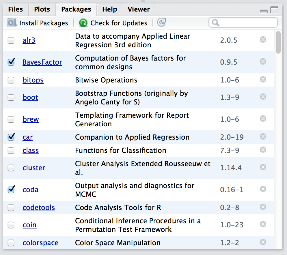
library() at the command line.
foreign package. The foreign package is a collection of tools that are very handy when R needs to interact with files that are produced by other software packages (e.g., SPSS). It comes bundled with R, so it’s one of the ones that you have installed already, but it won’t be one of the ones loaded. Inside the foreign package is a function called read.spss(). It’s a handy little function that you can use to import an SPSS data file into R, so let’s pretend we want to use it. Currently, the foreign package isn’t loaded, so if I ask R to tell me if it knows about a function called read.spss() it tells me that there’s no such thing...
exists( "read.spss" )
## [1] TRUE
foreign package, and check the box on the left hand side. The moment that you do this, you’ll see a command like this appear in the R console:
library("foreign", lib.loc="/Library/Frameworks/R.framework/Versions/3.0/Resources/library")
lib.loc bit will look slightly different on Macs versus on Windows, because that part of the command is just RStudio telling R where to look to find the installed packages. What I’ve shown you above is the Mac version. On a Windows machine, you’ll probably see something that looks like this:
library("foreign", lib.loc="C:/Program Files/R/R-3.0.2/library")
lib.loc bit is almost always unnecessary. Unless you’ve taken to installing packages in idiosyncratic places (which is something that you can do if you really want) R already knows where to look. So in the vast majority of cases, the command to load the foreign package is just this:
library("foreign")
library() commands. You don’t actually have to type them in yourself: you can use the RStudio package panel to do all your package loading for you. The only reason I include the library() commands sometimes is as a reminder to you to make sure that you have the relevant package loaded. Oh, and I suppose we should check to see if our attempt to load the package actually worked. Let’s see if R now knows about the existence of the read.spss() function...
exists( "read.spss" )
## [1] FALSE
foreign package, you’ll see this command appear on screen:
detach("package:foreign", unload=TRUE)
## Warning: 'foreign' namespace cannot be unloaded:
##   namespace 'foreign' is imported by 'rio', 'psych' so cannot be unloaded
read.spss() function still exists():
exists( "read.spss" )
## [1] FALSE
Matrix package, so let’s load that one and see what happens:
library( Matrix )
Loading required package: lattice
Matrix package makes use of some of the tools in the lattice package, and R has kept track of this dependency. So when you try to load the Matrix package, R recognises that you’re also going to need to have the lattice package loaded too. As a consequence, both packages get loaded, and R prints out a helpful little note on screen to tell you that it’s done so.
lattice package while the Matrix package is still loaded. This is easy enough to try: all I have to do is uncheck the box next to "lattice" in the packages panel. But if I try this, here’s what happens:
detach("package:lattice", unload=TRUE)
Error: package `lattice' is required by `Matrix' so will not be detached
Matrix and lattice, I need to do it in the correct order
car and psych. The car package is short for "Companion to Applied Regression" (which is a really great book, I’ll add), and it has a lot of tools that I’m quite fond of. The car package was written by a guy called John Fox, who has written a lot of great statistical tools for social science applications. The psych package was written by William Revelle, and it has a lot of functions that are very useful for psychologists in particular, especially in regards to psychometric techniques. For the most part, car and psych are quite unrelated to each other. They do different things, so not surprisingly almost all of the function names are different. But... there’s one exception to that. The car package and the psych package both contain a function called logit().logit(100), should R use the logit() function in the car package, or the one in the psych package? The answer is: R uses whichever package you loaded most recently, and it tells you this very explicitly. Here’s what happens when I load the car package, and then afterwards load the psych package:
library(car)
library(psych)
logit object (i.e., function) in the car package is no longer accessible to you. It’s been hidden (or "masked") from you by the one in the psych package.car package by using car::logit() as your command rather than logit(), since the car:: part tells R explicitly which package to use. See also ::: if you’re especially keen to force R to use functions it otherwise wouldn’t, but take care, since ::: can be dangerous.
install.packages() that you can use to do this. Even more conveniently, the RStudio team runs its own CRAN mirror and RStudio has a clean interface that lets you install packages without having to learn how to use the install.packages() command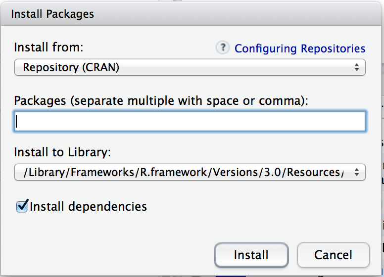
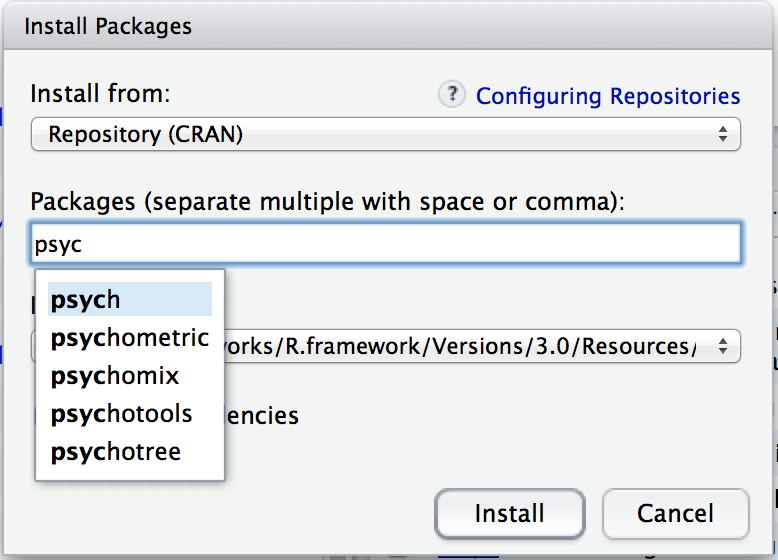
install.packages("psych")
install.packages() function is rather chatty, so it reports a bunch of gibberish that you really aren’t all that interested in:
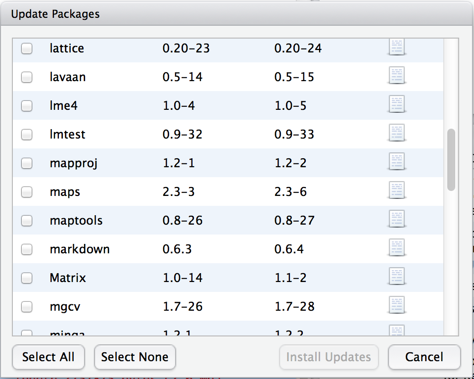
update.packages() function that you can use to do this, but it’s probably easier to stick with the RStudio tool. In the packages panel, click on the "Update Packages" button. This will bring up a window that looks like the one shown in Figure Figure 4.17. In this window, each row refers to a package that needs to be updated. You can to tell R which updates you want to install by checking the boxes on the left. If you’re feeling lazy and just want to update everything, click the "Select All" button, and then click the "Install Updates" button. R then prints out a lot of garbage on the screen, individually downloading and installing all the new packages. This might take a while to complete depending on how good your internet connection is. Go make a cup of coffee. Come back, and all will be well.
lsr. This is the Learning Statistics with R package that accompanies this book. It doesn’t have a lot of interesting high-powered tools: it’s just a small collection of handy little things that I think can be useful to novice users. As you get more comfortable with R this package should start to feel pretty useless to you.
psych. This package, written by William Revelle, includes a lot of tools that are of particular use to psychologists. In particular, there’s several functions that are particularly convenient for producing analyses or summaries that are very common in psych, but less common in other disciplines.
car. This is the Companion to Applied Regression package, which accompanies the excellent book of the same name by [42]. It provides a lot of very powerful tools, only some of which we’ll touch in this book.
gplots, sciplot, foreign, effects, R.matlab, gdata, lmtest, and probably one or two others that I’ve missed. There are also a number of packages that I refer to but don’t actually use in this book, such as reshape, compute.es, HistData and multcomp among others. Finally, there are a number of packages that provide more advanced tools that I hope to talk about in future versions of the book, such as sem, ez, nlme and lme4. In any case, whenever I’m using a function that isn’t in the core packages, I’ll make sure to note this in the text.
seeker, lover, and keeper. These three variables are the contents of your workspace, also referred to as the global environment. The workspace is a key concept in R, so in this section we’ll talk a lot about what it is and how to manage its contents.
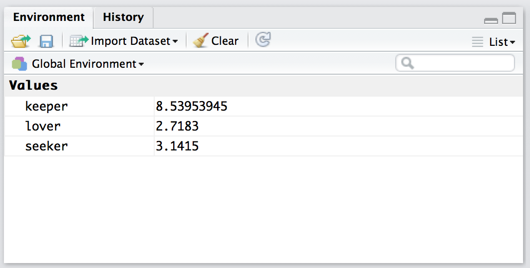
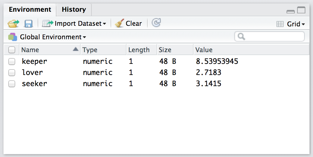
objects() function may come in handy:
objects()
## [1] "keeper" "lover" "seeker"
objects() function has a lot of fancy capabilities that I’m glossing over in this example. Moreover there are also several other functions that you can use, including ls() which is pretty much identical to objects(), and ls.str() which you can use to get a fairly detailed description of all the variables in the workspace. In fact, the lsr package actually includes its own function that you can use for this purpose, called who(). The reason for using the who() function is pretty straightforward: in my everyday work I find that the output produced by the objects() command isn’t quite informative enough, because the only thing it prints out is the name of each variable; but the ls.str() function is too informative, because it prints out a lot of additional information that I really don’t like to look at. The who() function is a compromise between the two. First, now that we’ve got the lsr package installed, we need to load it:
library(lsr)
who() function:
who()
##    -- Name --             -- Class --     -- Size --
##    keeper                 numeric         1
##    lover                  numeric         1
##    seeker                 numeric         1
who() function lists all the variables and provides some basic information about what kind of variable each one is and how many elements it contains. Personally, I find this output much easier more useful than the very compact output of the objects() function, but less overwhelming than the extremely verbose ls.str() function. Throughout this book you’ll see me using the who() function a lot. You don’t have to use it yourself: in fact, I suspect you’ll find it easier to look at the RStudio environment panel. But for the purposes of writing a textbook I found it handy to have a nice text based description: otherwise there would be about another 100 or so screenshots added to the book.who() function is searchable, whereas text shown in a screen shot isn’t!
who() command.
rm() comes in handy. The simplest way to use rm() is just to type in a (comma separated) list of all the variables you want to remove. Let’s say I want to get rid of seeker and lover, but I would like to keep keeper. To do this, all I have to do is type:
rm( seeker, lover )
who()
##    -- Name --             -- Class --     -- Size --
##    keeper                 numeric         1
keeper variable left. As you can see, rm() can be very handy for keeping the workspace tidy.
\ symbol. So, the complete path to this book on my Windows computer might be something like this: C:\Users\danRbook\LSR.pdf and what that means is that the book is called LSR.pdf, and it’s in a folder called book which itself is in a folder called dan which itself is ... well, you get the idea. On Linux, Unix and Mac OS systems, the addresses look a little different, but they’re more or less identical in spirit. Instead of using the backslash, folders are separated using a forward slash, and unlike Windows, they don’t treat the physical drive as being the root of the file system. So, the path to this book on my Mac might be something like this: /Users/dan/Rbook/LSR.pdf
C:\Users\dan or /Users/dan). That’s my current working directory.
. to refer to the current working directory, and .. to refer to the directory above it. This allows us to specify a path to a new location in relation to our current location, as the following examples illustrate. Let’s assume that I’m using my Windows computer, and my working directory is C:\Users\danRbook). The table below shows several addresses in relation to my current one:
knitr::kable(rbind(
                  c("C:\\\\Users\\\\dan" , ".."),
                  c("C:\\\\Users ", "..\\\\.. \\\\"),
                  c("C:\\\\Users\\\\danRbook\\\\source ", ".\\\\source "),
                  c("C:\\\\Users\\\\dan\\\\nerdstuff ", "..\\\\nerdstuff")),
caption = 'Basic arithmetic operations in R. These five operators are used very frequently throughout the text, so it\'s important to be familiar with them at the outset.',col.names = c("absolute path (i.e., from root)"  , "relative path (i.e. from C:\\Users\\danRbook)"),
  booktabs = TRUE)
~ directory. I normally wouldn’t bother, but R makes reference to this concept sometimes. It’s quite common on computers that have multiple users to define ~ to be the user’s home directory. On my Mac, for instance, the home directory ~ for the "dan" user is \Users\dan\. And so, not surprisingly, it is possible to define other directories in terms of their relationship to the home directory. For example, an alternative way to describe the location of the LSR.pdf file on my Mac would be
~Rbook\LSR.pdf
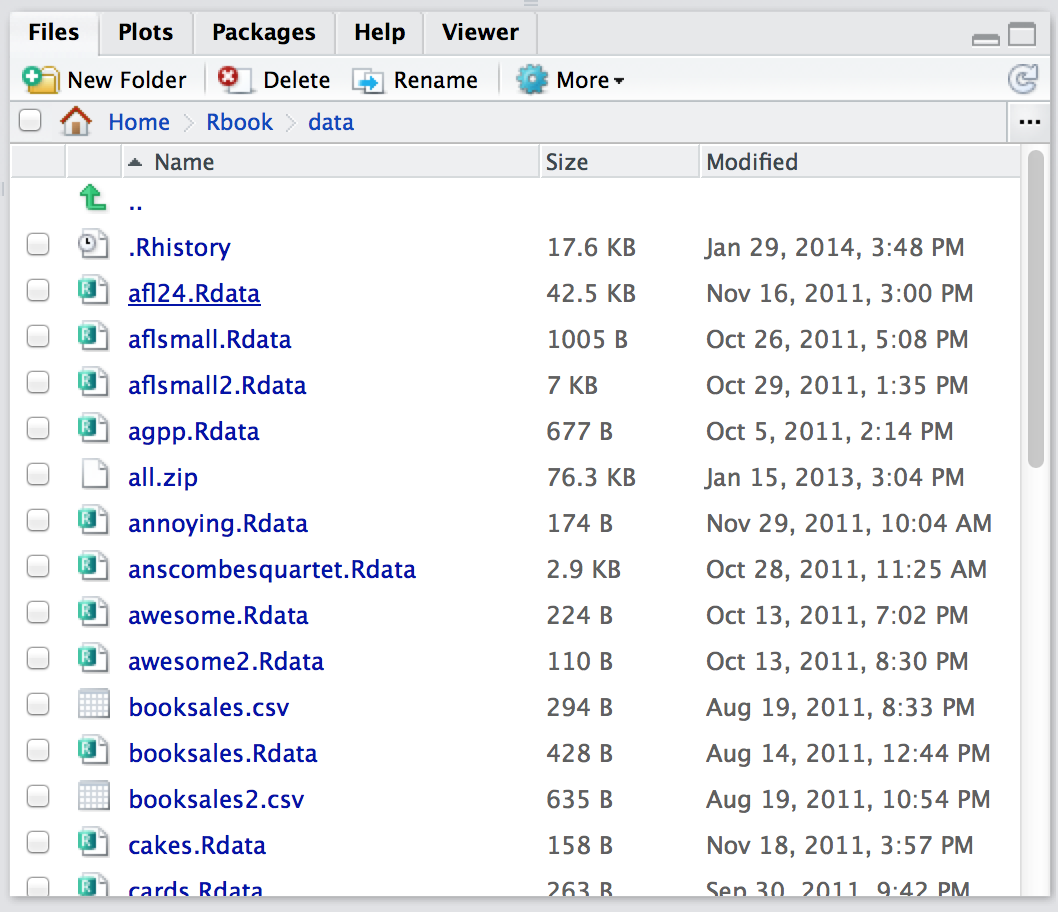
/Users/dan/Rbook/data
list.files() command to list the contents of the /Users/dan/Rbook/data directory (in Subsection 4.4.2), the output referred to a file called booksales.Rdata. Let’s say I want to load the data from this file into my workspace. The way I do this is with the load() function. There are two arguments to this function, but the only one we’re interested in is
file. This should be a character string that specifies a path to the file that needs to be loaded. You can use an absolute path or a relative path to do so.
load( file = "/Users/dan/Rbook/data/booksales.Rdata" )
/Users/dan/Rbook/data, I could use a relative file path, like so:
load( file = "../data/booksales.Rdata" )
setwd( "../data" )         # move to the data directory
load( "booksales.Rdata" )  # load the data
who() I’d see that there are several new variables in my workspace now. Throughout this book, whenever you see me loading a file, I will assume that the file is actually stored in the working directory, or that you’ve changed the working directory so that R is pointing at the directory that contains the file. Obviously, you don’t need type that command yourself: you can use the RStudio file panel to do the work.
booksales.Rdata file. All I have to do is click on the file name. RStudio brings up a little dialog box asking me to confirm that I do want to load this file. I click yes. The following command then turns up in the console,
load("~/Rbook/data/booksales.Rdata")
who()). So easy it barely warrants having its own section.
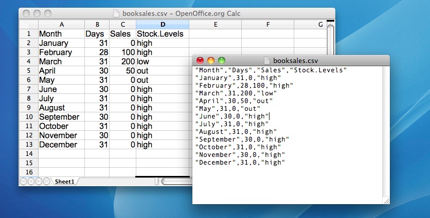
read.csv() function.read.table() function used for this purpose instead of read.csv(). They’re more or less identical functions, with the same arguments and everything. They differ only in the default values.
file. This should be a character string that specifies a path to the file that needs to be loaded. You can use an absolute path or a relative path to do so.
header. This is a logical value indicating whether or not the first row of the file contains variable names. The default value is TRUE.
books <- read.csv( file = "./data/booksales.csv" )
books <- read.csv( file = "booksales.csv" )
load() function, because that function is only meant to be used for .Rdata files. If you try to use load() on other types of data, you get an error. Secondly, notice that when I imported the CSV file I assigned the result to a variable, which I imaginatively called books..Rdata file is that it stores a whole workspace. So, if you had the ability to look inside the file yourself you’d see that the data file keeps track of all the variables and their names. So when you load() the file, R restores all those original names. CSV files are treated differently: as far as R is concerned, the CSV only stores one variable, but that variable is big table. So when you import that table into the workspace, R expects you to give it a name.] Let’s have a look at what we’ve got:
print( books )
##        Month Days Sales Stock.Levels
## 1    January   31     0         high
## 2   February   28   100         high
## 3      March   31   200          low
## 4      April   30    50          out
## 5        May   31     0          out
## 6       June   30     0         high
## 7       July   31     0         high
## 8     August   31     0         high
## 9  September   30     0         high
## 10   October   31     0         high
## 11  November   30     0         high
## 12  December   31     0         high
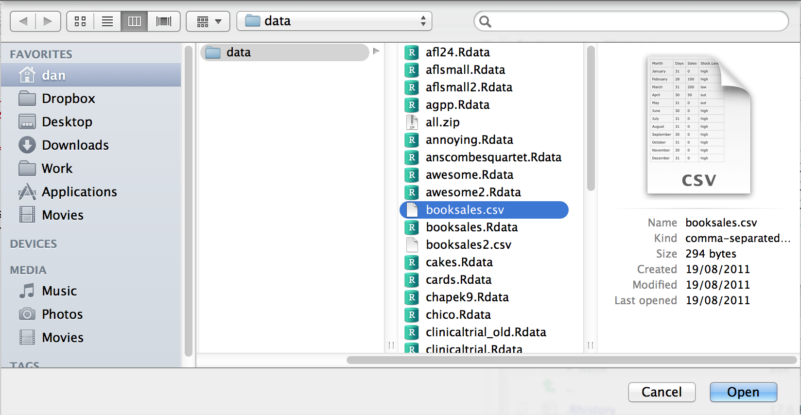
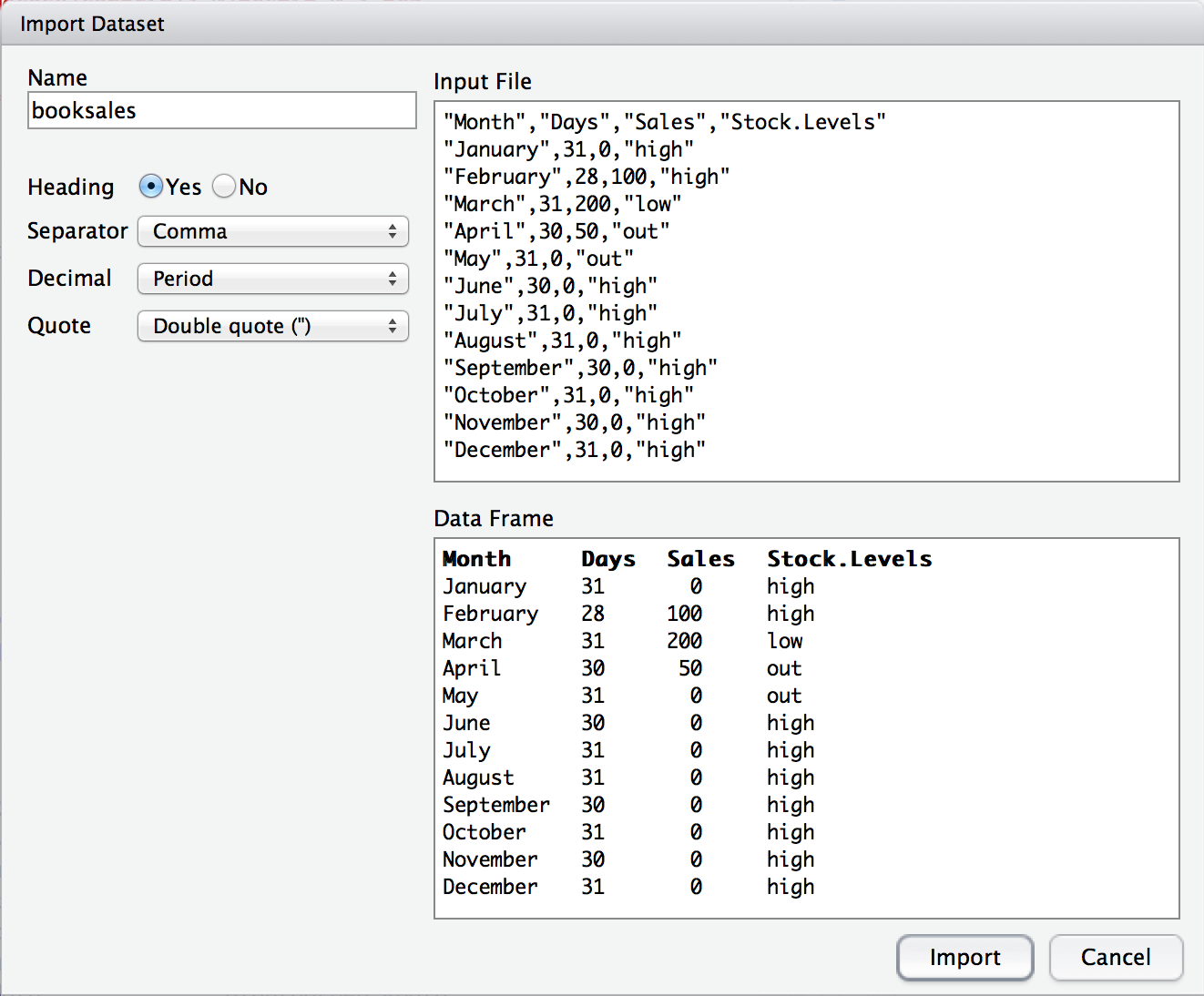
booksales.csv, so RStudio suggests the name booksales. If you’re happy with that, leave it alone. If not, type something else. Immediately below this are a few things that you can tweak to make sure that the data gets imported correctly:
booksales.csv file has a header at the top, so I selected "yes".
.). That’s not universally true: many European countries use a comma. So you can change that if you need to.
booksales.csv file, so that’s what I selected.
booksales <- read.csv("~/Rbook/data/booksales.csv")
View(booksales)
save
save() and save.image(). If you’re happy to save all of the variables in your workspace into the data file, then you should use save.image(). And if you’re happy for R to save the file into the current working directory, all you have to do is this:
save.image( file = "myfile.Rdata" )
file is the first argument, you can shorten this to save.image("myfile.Rdata"); and if you want to save to a different directory, then (as always) you need to be more explicit about specifying the path to the file, just as we discussed in Section 4.4. Suppose, however, I have several variables in my workspace, and I only want to save some of them. For instance, I might have this as my workspace:
who()
-- Name --   -- Class --   -- Size --
data         data.frame    3 x 2
handy        character     1
junk         numeric       1
data and handy, but not junk. But I don’t want to delete junk right now, because I want to use it for something else later on. This is where the save() function is useful, since it lets me indicate exactly which variables I want to save. Here is one way I can use the save function to solve my problem:
save(data, handy, file = "myfile.Rdata")
file argument. The reason is that if you don’t do so, R will think that "myfile.Rdata" is actually a variable that you want to save, and you’ll get an error message. Finally, I should mention a second way to specify which variables the save() function should save, which is to use the list argument. You do so like this:
save.me <- c("data", "handy")   # the variables to be saved
save( file = "booksales2.Rdata", list = save.me )   # the command to save them
.R files. We won’t get to those until Chapter 8.
save.image("~/Desktop/Untitled.RData")
sink()), but to be honest, if you do want to save the R output, the easiest thing to do is to use the mouse to select the relevant text in the R console, go to the "Edit" menu in RStudio and select "Copy". The output has now been copied to the clipboard. Now open up your favourite text editor or word processing software, and paste it. And you’re done. However, this will only save the contents of the console, not the plots you’ve drawn (assuming you’ve drawn some). We’ll talk about saving images later on.
Inf, NaN, NA and NULL. These values can crop up in various different places, and so it’s important to understand what they mean.
Inf). The easiest of the special values to explain is Inf, since it corresponds to a value that is infinitely large. You can also have -Inf. The easiest way to get Inf is to divide a positive number by 0:
1 / 0
## [1] Inf
NaN). The special value of NaN is short for "not a number", and it’s basically a reserved keyword that means "there isn’t a mathematically defined number for this". If you can remember your high school maths, remember that it is conventional to say that $0/0$ doesn’t have a proper answer: mathematicians would say that $0/0$ is undefined. R says that it’s not a number:
0 / 0
## [1] NaN
NaN corresponds to cases where you asked a proper numerical question that genuinely has no meaningful answer.
NA).
NA indicates that the value that is "supposed" to be stored here is missing. To understand what this means, it helps to recognise that the NA value is something that you’re most likely to see when analysing data from real world experiments. Sometimes you get equipment failures, or you lose some of the data, or whatever. The point is that some of the information that you were "expecting" to get from your study is just plain missing. Note the difference between NA and NaN. For NaN, we really do know what’s supposed to be stored; it’s just that it happens to correspond to something like $0/0$ that doesn’t make any sense at all. In contrast, NA indicates that we actually don’t know what was supposed to be there. The information is missing.
NULL).
NULL value takes this "absence" concept even further. It basically asserts that the variable genuinely has no value whatsoever. This is quite different to both NaN and NA. For NaN we actually know what the value is, because it’s something insane like $0/0$. For NA, we believe that there is supposed to be a value "out there", but a dog ate our homework and so we don’t quite know what it is. But for NULL we strongly believe that there is no value at all.
profit <- c( 3.1, 0.1, -1.4, 1.1 )
profit
## [1] 3.1 0.1 -1.4 1.1
names to each of the elements. Here’s how you do it:
names(profit) <- c("Q1","Q2","Q3","Q4")
profit
##   Q1   Q2   Q3   Q4
##  3.1  0.1 -1.4  1.1
names(profit). You can always delete the names again by using the command names(profit) <- NULL. It’s also worth noting that you don’t have to do this as a two stage process. You can get the same result with this command:
profit <- c( "Q1" = 3.1, "Q2" = 0.1, "Q3" = -1.4, "Q4" = 1.1 )
profit
##   Q1   Q2   Q3   Q4
##  3.1  0.1 -1.4  1.1
profit[1] is still 3.1; all I’ve done is added a name to profit[1] as well. Nevertheless, names aren’t purely cosmetic, since R allows you to pull out particular elements of the vector by referring to their names:
profit["Q1"]
##  Q1
## 3.1
names(profit).
x <- 5   # x is numeric
y <- 4   # y is numeric
x * y
## [1] 20
x <- "apples"   # x is character
y <- "oranges"  # y is character
x * y
## Error in x * y: non-numeric argument to binary operator
"apples" by "oranges". It knows this because the quote marks are indicators that the variable is supposed to be treated as text, not as a number.
5 and "5". Without quote marks, R treats 5 as the number five, and will allow you to do calculations with it. With the quote marks, R treats "5" as the textual character five, and doesn’t recognise it as a number any more than it recognises "p" or "five" as numbers. As a consequence, there’s a big difference between typing x <- 5 and typing x <- "5". In the former, we’re storing the number 5; in the latter, we’re storing the character "5". Thus, if we try to do multiplication with the character versions, R gets stroppy:
x <- "5"   # x is character
y <- "4"   # y is character
x * y
## Error in x * y: non-numeric argument to binary operator
x (which happens depressingly often). R provides a function that will let us find out. Or, more precisely, it provides three functions: class(), mode() and typeof(). Why the heck does it provide three functions, you might be wondering? Basically, because R actually keeps track of three different kinds of information about a variable:
"2011-09-12" and "my birthday" are both text strings, but there’s an important difference between the two: one of them is a date. So it would be nice if we could get R to recognise that "2011-09-12" is a date, and allow us to do things like add or subtract from it. The class of a variable is what R uses to keep track of things like that. Because the class of a variable is critical for determining what R can or can’t do with it, the class() function is very handy.
mode() function very much.typeof() function.
class() of the variable that we care most about. Later on, I’ll talk a bit about how you can convince R to "coerce" a variable to change from one class to another (Section 7.10). That’s a useful skill for real world data analysis, but it’s not something that we need right now. In the meantime, the following examples illustrate the use of the class() function:
x <- "hello world"     # x is text
class(x)


x <- TRUE     # x is logical
class(x)

x <- 100     # x is a number
class(x)
## [1] "character"
RT <- c(342, 401, 590, 391, 554)
2 * RT

RT + 1000
## [1]  684  802 1180  782 1108
## [1] 1342 1401 1590 1391 1554
group <- c(1,1,1,2,2,2,3,3,3)
group[i] contains the group membership of the i-th person in my study. Clearly, this is numeric data, but equally obviously this is a nominal scale variable. There’s no sense in which "group 1" plus "group 2" equals "group 3", but nevertheless if I try to do that, R won’t stop me because it doesn’t know any better:
group + 2
## [1] 3 3 3 4 4 4 5 5 5
3 is an ordinary number in this context, so it sees no problem in calculating 3 + 2. But since we’re not that stupid, we’d like to stop R from doing this. We can do so by instructing R to treat group as a factor. This is easy to do using the as.factor() function.group <- as.factor(group)
group
## [1] 1 1 1 2 2 2 3 3 3
## Levels: 1 2 3
Levels rubbish is about), but if we ask R to tell us what the class of the group variable is now, it’s clear that it has done what we asked:
class(group)
## [1] "factor"
group to a factor, look what happens when I try to add 2 to it:
group + 2
## [1] 3 3 3 4 4 4 5 5 5
NA: see Subsection 4.6.1).
gender, with two levels corresponding to males and females. But when I go to print out the variable I get something like this:
gender<-as.factor(c(1, 1 ,1, 1 ,1, 2 ,2, 2 , 2))
## [1] 1 1 1 1 1 2 2 2 2
## Levels: 1 2
gender
## [1] 1 1 1 1 1 2 2 2 2
## Levels: 1 2
levels(group) <- c("group 1", "group 2", "group 3")
print(group)

levels(gender) <- c("male", "female")
print(gender)
## [1] 1 1 1 1 1 2 2 2 2
## Levels: 1 2
rm(books, keeper, profit, RT, x, y)
group and gender for all 9 participants in my study. Let’s also suppose I recorded their ages and their score on "Dan’s Terribly Exciting Psychological Test":
age <- c(17, 19, 21, 37, 18, 19, 47, 18, 19)
score <- c(12, 10, 11, 15, 16, 14, 25, 21, 29)
## Error in eval(expr, envir, enclos): object 'score' not found
who() I get this:
who()
##    -- Name --             -- Class --     -- Size --
##    age                    numeric         9
##    gender                 factor          9
##    group                  factor          9
##    score                  numeric         9
age, gender, group and score. And it just so happens that all four of them are the same size (i.e., they’re all vectors with 9 elements). Aaaand it just so happens that age[1] corresponds to the age of the first person, and gender[1] is the gender of that very same person, etc. In other words, you and I both know that all four of these variables correspond to the same data set, and all four of them are organised in exactly the same way.
age variable has to be the same length as the gender variable; and there’s no particular reason to think that age[1] has any special relationship to gender[1] any more than it has a special relationship to gender[4]. In other words, when we store everything in separate variables like this, R doesn’t know anything about the relationships between things. It doesn’t even really know that these variables actually refer to a proper data set. The data frame fixes this: if we store our variables inside a data frame, we’re telling R to treat these variables as a single, fairly coherent data set.
data.frame() function. All you have to do is type a list of variables that you want to include in the data frame. The output of a data.frame() command is, well, a data frame. So, if I want to store all four variables from my experiment in a data frame called expt I can do so like this:
expt <- data.frame ( age, gender, group, score )
expt
##   age gender   group score
## 1  17   male group 1    12
## 2  19   male group 1    10
## 3  21   male group 1    11
## 4  37   male group 2    15
## 5  18   male group 2    16
## 6  19 female group 2    14
## 7  47 female group 3    25
## 8  18 female group 3    21
## 9  19 female group 3    29
expt is a completely self-contained variable. Once you’ve created it, it no longer depends on the original variables from which it was constructed. That is, if we make changes to the original age variable, it will not lead to any changes to the age data stored in expt.
$
expt. But as we can see when we told R to print the variable out, this data frame contains 4 variables, each of which has 9 observations. So how do we get this information out again? After all, there’s no point in storing information if you don’t use it, and there’s no way to use information if you can’t access it. So let’s talk a bit about how to pull information out of a data frame.
score. One thing you might try to do is ignore the fact that score is locked up inside the expt data frame. For instance, you might try to print it out like this:
score
Error: object 'score' not found
$ operator to extract the variable you’re interested in, like this:
expt$score
## [1] 12 10 11 15 16 14 25 21 29
objects() or who(), but neither of those commands will tell you what the names are for those variables inside a data frame! One way is to ask R to tell you what the names of all the variables stored in the data frame are, which you can do using the names() function:
names(expt)
## [1] "age" "gender" "group" "score"
who() function, as long as you tell it to look at the variables inside data frames. If you set expand = TRUE then it will not only list the variables in the workspace, but it will "expand" any data frames that you’ve got in the workspace, so that you can see what they look like. That is:
who(expand = TRUE)
##    -- Name --             -- Class --     -- Size --
##    expt                   data.frame      9 x 4
##    $age                   numeric         9
##    $gender                factor          9
##    $group                 factor          9
##    $score                 numeric         9
expand is the first argument in the who() function you can just type who(TRUE). I’ll do that a lot in this book.
list() function. If I type this as my command:
Dan <- list( age = 34,
            nerd = TRUE,
            parents = c("Joe","Liz")
)
Dan, which is a bundle of three different variables: age, nerd and parents. Notice, that the parents variable is longer than the others. This is perfectly acceptable for a list, but it wouldn’t be for a data frame. If we now print out the variable, you can see the way that R stores the list:
print( Dan )
## $age
## [1] 34
##
## $nerd
## [1] TRUE
##
## $parents
## [1] "Joe" "Liz"
$ symbols everywhere, the variables are stored in exactly the same way that they are for a data frame (again, this is not surprising: data frames are a type of list). So you will (I hope) be entirely unsurprised and probably quite bored when I tell you that you can extract the variables from the list using the $ operator, like so:
Dan$nerd
## [1] TRUE
$, as the following example illustrates. If I type a command like this
Dan$children <- "Alex"
children, and assigns it a value of "Alex". If I were now to print() this list out, you’d see a new entry at the bottom of the printout. Finally, it’s actually possible for lists to contain other lists, so it’s quite possible that I would end up using a command like Dan$children$age to find out how old my son is. Or I could try to remember it myself I suppose.
~. A very simple example of a formula is shown below:out and pred variables actually exist: it’s only later on when you try to use the formula for something that this happens.
formula1 <- out ~ pred
formula1
## out ~ pred
out (outcome) variable, analysed in terms of the pred (predictor) variable". That said, although the simplest and most common form of a formula uses the "one variable on the left, one variable on the right" format, there are others. For instance, the following examples are all reasonably common
formula2 <-  out ~ pred1 + pred2   # more than one variable on the right
formula3 <-  out ~ pred1 * pred2   # different relationship between predictors
formula4 <-  ~ var1 + var2         # a 'one-sided' formula
summary() and plot(), although you’ve already seen an example of one working behind the scenes, and that’s the print() function. The thing that makes generics different from the other functions is that their behaviour changes, often quite dramatically, depending on the class() of the input you give it. The easiest way to explain the concept is with an example. With that in mind, lets take a closer look at what the print() function actually does. I’ll do this by creating a formula, and printing it out in a few different ways. First, let’s stick with what we know:
my.formula <- blah ~ blah.blah    # create a variable of class "formula"
print( my.formula )               # print it out using the generic print() function
## blah ~ blah.blah
print( my.formula ), what actually happens is the print() function checks the class of the my.formula variable. When the function discovers that the variable it’s been given is a formula, it goes looking for a function called print.formula(), and then delegates the whole business of printing out the variable to the print.formula() function.print.formula() that exists only to be a special case of a generic function like print() is a method, and the name for the process in which the generic function passes off all the hard work onto a method is called method dispatch. You won’t need to understand the details at all for this book, but you do need to know the gist of it; if only because a lot of the functions we’ll use are actually generics. Anyway, to help expose a little more of the workings to you, let’s bypass the print() function entirely and call the formula method directly:
print.formula( my.formula ) # print it out using the print.formula() method
blah ~ blah.blah
print.formula() method that was doing all the hard work in the first place. The print() function itself is a lazy bastard that doesn’t do anything other than select which of the methods is going to do the actual printing.
print.formula() didn’t exist? That is, what happens if there isn’t a specific method defined for the class of variable that you’re using? In that case, the generic function passes off the hard work to a "default" method, whose name in this case would be print.default(). Let’s see what happens if we bypass the print() formula, and try to print out my.formula using the print.default() function:
print.default( my.formula ) # print it out using the print.default() method
## blah ~ blah.blah
## attr(,"class")
## [1] "formula"
## attr(,".Environment")
## <environment: R_GlobalEnv>
print.default() method doesn’t know anything about formulas, and doesn’t know that it’s supposed to be hiding the obnoxious internal gibberish that R produces sometimes.
load() function. To do so, I type either of the following:
?load
help("load")
??load
help.search("load")
load" topic as our example. Firstly, at the very top we see this:
load {base} R Documentation
load { base } part is telling you that this is in reference to the load() function (obviously) and that this function is in the base package. Next, we get the "title" information, and a short "description" of what the function does:
Reload Saved Datasets
Description:
Reload datasets written with the function save.
Usage:
load(file, envir = parent.frame(), verbose = FALSE)
load() function: the first one is called file, and the second one is called envir. It’s also telling you that there is a default value for the envir argument; so if the user doesn’t specify what the value of envir should be, then R will assume that envir = parent.frame(). In contrast, the file argument has no default value at all, so the user must specify a value for it. So in one sense, this section is very straightforward.
parent.frame() function actually does, so it’s hard for you to know what the envir = parent.frame() bit is all about. What you could do is then go look up the help documents for the parent.frame() function (and sometimes that’s actually a good idea), but often you’ll find that the help documents for those functions are just as dense (if not more dense) than the help file that you’re currently reading. As an alternative, my general approach when faced with something like this is to skim over it, see if I can make any sense of it. If so, great. If not, I find that the best thing to do is ignore it. In fact, the first time I read the help file for the load() function, I had no idea what any of the envir related stuff was about. But fortunately I didn’t have to: the default setting here (i.e., envir = parent.frame()) is actually the thing you want in about 99% of cases, so it’s safe to ignore it.
file a (readable binary-mode) connection or a character string giving the name of the file to load (when tilde expansion is done).
envir the environment where the data should be loaded.
file argument needs to be a string (i.e., text data) which tells R the name of the file to load. It also seems to be hinting that there’s other possibilities too (e.g., a “binary mode connection”), and you probably aren’t quite sure what “tilde expansion” meansenvir argument, it’s now a little clearer what the Usage section was babbling about. The envir argument specifies the name of an environment (see Section 4.3 if you’ve forgotten what environments are) into which R should place the variables when it loads the file. Almost always, this is a no-brainer: you want R to load the data into the same damn environment in which you’re invoking the load() command. That is, if you’re typing load() at the R prompt, then you want the data to be loaded into your workspace (i.e., the global environment). But if you’re writing your own function that needs to load some data, you want the data to be loaded inside that function’s private workspace. And in fact, that’s exactly what the parent.frame() thing is all about. It’s telling the load() function to send the data to the same place that the load() command itself was coming from. As it turns out, if we’d just ignored the envir bit we would have been totally safe. Which is nice to know.
load can load R objects saved in the current or any earlier
"rb" and closed
1971:1977 are from R <
RD[ABX]1 from R 0.99.0 to R 1.3.1. These are all
verbose argument is mainly intended for debugging. If it
TRUE, then as objects from the file are loaded, their
verbose is set to
load() function is mainly used to load variables into the workspace rather than to return a value, it’s no surprise that this doesn’t do much or say much. Moving on, we sometimes see a few additional sections in the help file, which can be different depending on what the function is:
ascii = TRUE, so ensure that they are transferred without
load tries to detect such a
load(<file>) replaces all existing objects with the same names
envir = to load into a
load()s into a new entry in the search path.
file can be a UTF-8-encoded filepath that cannot be translated to
load().
load" help file:
load() function, so it’s not a bad idea to have a look at them, and to try not to find them too intimidating.
help.request() function that R provides to check that you’re actually doing what you’re expected.


Remark 4.1. R Code.