load( "./data/aflsmall.Rdata" )
library(lsr)
who()
##    -- Name --             -- Class --     -- Size --
##    afl.finalists          factor          400
##    afl.margins            numeric         176
aflsmall.Rdata file, and use the who() function in the lsr package to see what variables are stored in the file:
load( "./data/aflsmall.Rdata" )
library(lsr)
who()
## -- Name -- -- Class -- -- Size -- ## afl.finalists factor 400 ## afl.margins numeric 176
afl.finalists and afl.margins. We’ll focus a bit on these two variables in this chapter, so I’d better tell you what they are. Unlike most of data sets in this book, these are actually real data, relating to the Australian Football League (AFL) afl.margins variable contains the winning margin (number of points) for all 176 home and away games played during the 2010 season. The afl.finalists variable contains the names of all 400 teams that played in all 200 finals matches played during the period 1987 to 2010. Let’s have a look at the afl.margins variable:
print(afl.margins)
##   [1]  56  31  56   8  32  14  36  56  19   1   3 104  43  44  72   9  28
##  [18]  25  27  55  20  16  16   7  23  40  48  64  22  55  95  15  49  52
##  [35]  50  10  65  12  39  36   3  26  23  20  43 108  53  38   4   8   3
##  [52]  13  66  67  50  61  36  38  29   9  81   3  26  12  36  37  70   1
##  [69]  35  12  50  35   9  54  47   8  47   2  29  61  38  41  23  24   1
##  [86]   9  11  10  29  47  71  38  49  65  18   0  16   9  19  36  60  24
## [103]  25  44  55   3  57  83  84  35   4  35  26  22   2  14  19  30  19
## [120]  68  11  75  48  32  36  39  50  11   0  63  82  26   3  82  73  19
## [137]  33  48   8  10  53  20  71  75  76  54  44   5  22  94  29   8  98
## [154]   9  89   1 101   7  21  52  42  21 116   3  44  29  27  16   6  44
## [171]   3  28  38  29  10  10
afl.margins data, since it should help you get a sense of what the data we’re trying to describe actually look like. But for what it’s worth, this histogram — which is shown in Figure 5.3 — was generated using the hist() function. We’ll talk a lot more about how to draw histograms in Section 6.3. For now, it’s enough to look at the histogram and note that it provides a fairly interpretable representation of the afl.margins data.
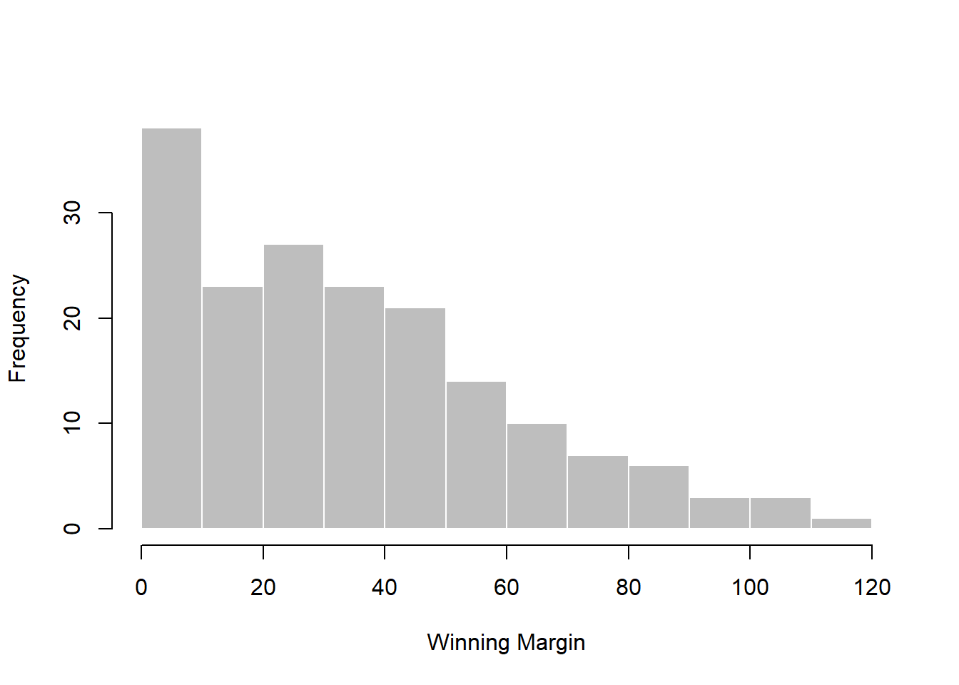
afl.margins variable). As you might expect, the larger the margin the less frequently you tend to see it.afl.margins variable, along with the mathematical symbol used to refer to it, and the actual value that the observation corresponds to:
| the observation | its symbol | the observed value |
|---|---|---|
| winning margin, game 1 | \(X_1\) | 56 points |
| winning margin, game 2 | \(X_2\) | 31 points |
| winning margin, game 3 | \(X_3\) | 56 points |
| winning margin, game 4 | \(X_4\) | 8 points |
| winning margin, game 5 | \(X_5\) | 32 points |
(56 + 31 + 56 + 8 + 32) / 5
## [1] 36.6
afl.margins variable. Under those circumstances, what you want is a function that will just add up all the values stored in a numeric vector. That’s what the sum() function does. If we want to add up all 176 winning margins in the data set, we can do so using the following command:c() and the remove function rm(), the sum() function has unnamed arguments. I’ll talk about unnamed arguments later in Subsection 8.4.1, but for now let’s just ignore this detail.
sum( afl.margins )
## [1] 6213
sum( afl.margins[1:5] )
## [1] 183
sum( afl.margins[1:5] ) / 5
## [1] 36.6
sum() function, we can do it in an even easier way, since R also provides us with the mean() function. To calculate the mean for all 176 games, we would use the following command:
mean( x = afl.margins )
## [1] 35.30114
x is the first argument to the function, I could have omitted the argument name. In any case, just to show you that there’s nothing funny going on, here’s what we would do to calculate the mean for the first five observations:
mean( afl.margins[1:5] )
## [1] 36.6
sort() function (discussed in Chapter 7) to display the winning margins in increasing numerical order:sort( x = afl.margins )
##   [1]   0   0   1   1   1   1   2   2   3   3   3   3   3   3   3   3   4
##  [18]   4   5   6   7   7   8   8   8   8   8   9   9   9   9   9   9  10
##  [35]  10  10  10  10  11  11  11  12  12  12  13  14  14  15  16  16  16
##  [52]  16  18  19  19  19  19  19  20  20  20  21  21  22  22  22  23  23
##  [69]  23  24  24  25  25  26  26  26  26  27  27  28  28  29  29  29  29
##  [86]  29  29  30  31  32  32  33  35  35  35  35  36  36  36  36  36  36
## [103]  37  38  38  38  38  38  39  39  40  41  42  43  43  44  44  44  44
## [120]  44  47  47  47  48  48  48  49  49  50  50  50  50  52  52  53  53
## [137]  54  54  55  55  55  56  56  56  57  60  61  61  63  64  65  65  66
## [154]  67  68  70  71  71  72  73  75  75  76  81  82  82  83  84  89  94
## [171]  95  98 101 104 108 116
median( x = afl.margins )
## [1] 30.5
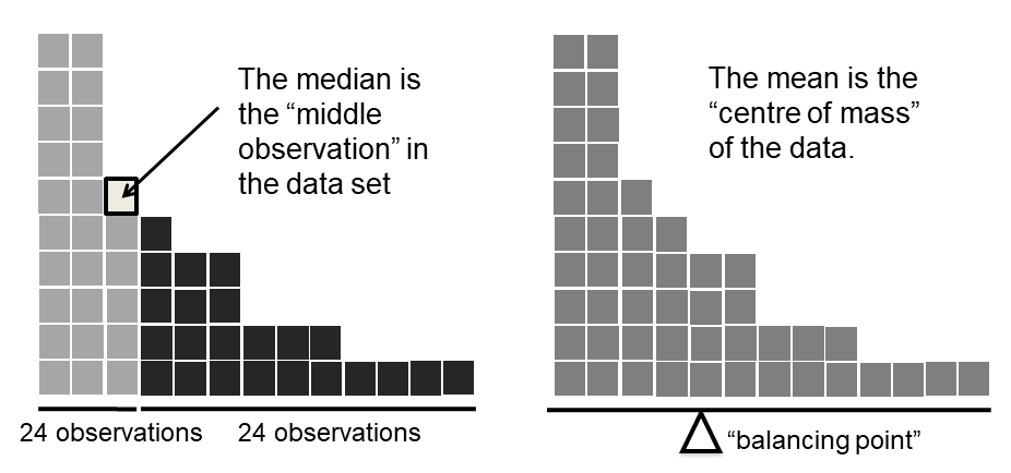
Senior Commonwealth Bank executives have travelled the world in the past couple of weeks with a presentation showing how Australian house prices, and the key price to income ratios, compare favourably with similar countries. "Housing affordability has actually been going sideways for the last five to six years," said Craig James, the chief economist of the bank’s trading arm, CommSec.
CBA has waged its war against what it believes are housing doomsayers with graphs, numbers and international comparisons. In its presentation, the bank rejects arguments that Australia’s housing is relatively expensive compared to incomes. It says Australia’s house price to household income ratio of 5.6 in the major cities, and 4.3 nationwide, is comparable to many other developed nations. It says San Francisco and New York have ratios of 7, Auckland’s is 6.7, and Vancouver comes in at 9.3.
Many analysts say that has led the bank to use misleading figures and comparisons. If you go to page four of CBA’s presentation and read the source information at the bottom of the graph and table, you would notice there is an additional source on the international comparison — Demographia. However, if the Commonwealth Bank had also used Demographia’s analysis of Australia’s house price to income ratio, it would have come up with a figure closer to 9 rather than 5.6 or 4.3
[An] obvious problem with the Commonwealth Bank’s domestic price to income figures is they compare average incomes with median house prices (unlike the Demographia figures that compare median incomes to median prices). The median is the mid-point, effectively cutting out the highs and lows, and that means the average is generally higher when it comes to incomes and asset prices, because it includes the earnings of Australia’s wealthiest people. To put it another way: the Commonwealth Bank’s figures count Ralph Norris’ multi-million dollar pay packet on the income side, but not his (no doubt) very expensive house in the property price figures, thus understating the house price to income ratio for middle-income Australians.
[As] Australia’s largest home lender, the Commonwealth Bank has one of the biggest vested interests in house prices rising. It effectively owns a massive swathe of Australian housing as security for its home loans as well as many small business loans.
12) and the smallest value (i.e., -15) and taking the mean of the remaining values. First, let’s enter the data
dataset <- c( -15,2,3,4,5,6,7,8,9,12 )
mean( x = dataset )

median( x = dataset )
## [1] 4.1
## [1] 5.5
mean( x = dataset, trim = .1)
## [1] 5.5
trim = .1, not trim = 10. In any case, let’s finish up by calculating the 5% trimmed mean for the afl.margins data,
mean( x = afl.margins, trim = .05)
## [1] 33.75
afl.finalists variable is a factor that contains the name of every team that played in any AFL final from 1987-2010, so let’s have a look at it. To do this we will use the head() command. head() is useful when you’re working with a data.frame with a lot of rows since you can use it to tell you how many rows to return. There have been a lot of finals in this period so printing afl.finalists using print(afl.finalists) will just fill us the screen. The command below tells R we just want the first 25 rows of the data.frame.
head(afl.finalists, 25)
##  [1] Hawthorn    Melbourne   Carlton     Melbourne   Hawthorn
##  [6] Carlton     Melbourne   Carlton     Hawthorn    Melbourne
## [11] Melbourne   Hawthorn    Melbourne   Essendon    Hawthorn
## [16] Geelong     Geelong     Hawthorn    Collingwood Melbourne
## [21] Collingwood West Coast  Collingwood Essendon    Collingwood
## 17 Levels: Adelaide Brisbane Carlton Collingwood Essendon ... Western Bulldogs
table() function (discussed in more detail in Section 7.1) to do this task for us:
table( afl.finalists )
## afl.finalists
##         Adelaide         Brisbane          Carlton      Collingwood
##               26               25               26               28
##         Essendon          Fitzroy        Fremantle          Geelong
##               32                0                6               39
##         Hawthorn        Melbourne  North Melbourne    Port Adelaide
##               27               28               28               17
##         Richmond         St Kilda           Sydney       West Coast
##                6               24               26               38
## Western Bulldogs
##               24
finalists data is "Geelong". The core packages in R don’t have a function for calculating the modemode(), but it does something completely different.
lsr package that does this. The function is called modeOf(), and here’s how you use it:
modeOf( x = afl.finalists )
## [1] "Geelong"
maxFreq() that tells you what the modal frequency is. If we apply this function to our finalists data, we obtain the following:
maxFreq( x = afl.finalists )
## [1] 39
afl.margins variable. This variable is clearly ratio scale (if it’s not clear to you, it may help to re-read Section 2.2), and so in most situations the mean or the median is the measure of central tendency that you want. But consider this scenario... a friend of yours is offering a bet. They pick a football game at random, and (without knowing who is playing) you have to guess the exact margin. If you guess correctly, you win $50. If you don’t, you lose $1. There are no consolation prizes for "almost" getting the right answer. You have to guess exactly the right marginmodeOf( x = afl.margins )
maxFreq( x = afl.margins )
## [1] 3
## [1] 8
afl.margins data. We’ll use this data to discuss several different measures of spread, each with different strengths and weaknesses.
max() and min() functions:
max( afl.margins )
min( afl.margins )
range() function; which outputs both the minimum value and the maximum value in a vector, like this:
range( afl.margins )
## [1] 0 116
quantile() function. Let’s use it to calculate the median AFL winning margin:
quantile( x = afl.margins, probs = .5)
##  50%
## 30.5
median() function. Now, we can actually input lots of quantiles at once, by specifying a vector for the probs argument. So lets do that, and get the 25th and 75th percentile:
quantile( x = afl.margins, probs = c(.25,.75) )
##   25%   75%
## 12.75 50.50
IQR() that we can use:
IQR( x = afl.margins )
## [1] 37.75
abs() function in R (Section 3.5), we do this by converting any negative values to positive ones. Mathematically, we would denote the absolute value of \(-3\) as \(|-3|\text{,}\) and so we say that \(|-3| = 3\text{.}\) We use the absolute value function here because we don’t really care whether the value is higher than the mean or lower than the mean, we’re just interested in how close it is to the mean. To help make this process as obvious as possible, the table below shows these calculations for all five observations:
| game | symbol | value \(X_i\) | deviation \(X_i - \bar{X}\) | absolute deviation \(\lvert X_i - \bar{X} \rvert\) |
|---|---|---|---|---|
| game 1 | \(X_1\) | 56 | 19.4 | 19.4 |
| game 2 | \(X_2\) | 31 | -5.6 | 5.6 |
| game 3 | \(X_3\) | 56 | 19.4 | 19.4 |
| game 4 | \(X_4\) | 8 | -28.6 | 28.6 |
| game 5 | \(X_5\) | 32 | -4.6 | 4.6 |
X <- c(56, 31,56,8,32)   # enter the data
X.bar <- mean( X )       # step 1. the mean of the data
AD <- abs( X - X.bar )   # step 2. the absolute deviations from the mean
AAD <- mean( AD )        # step 3. the mean absolute deviations
print( AAD )             # print the results
## [1] 15.52
lsr package has a very simple function called aad() that does the calculations for you. If we apply the aad() function to our data, we get this:
library(lsr)
aad( X )
## [1] 15.52
| Notation [English] | \(i\) [which game] | \(X_i\) [value] | \(X_i - \bar{X}\) [deviation from mean] | \((X_i - \bar{X})^2\) [absolute deviation] |
|---|---|---|---|---|
| 1 | 56 | 19.4 | 376.36 | |
| 2 | 31 | -5.6 | 31.36 | |
| 3 | 56 | 19.4 | 376.36 | |
| 4 | 8 | -28.6 | 817.96 | |
| 5 | 32 | -4.6 | 21.16 |
( 376.36 + 31.36 + 376.36 + 817.96 + 21.16 ) / 5
## [1] 324.64
X lying around, which we created in the previous section. With this in mind, we can calculate the variance of X by using the following command,
mean( (X - mean(X) )^2)
## [1] 324.64
var() which does calculate variances. So we could also do this...
var(X)
## [1] 405.8
afl.margins vector. First, let’s calculate the variance by using the formula that I described above:
mean( (afl.margins - mean(afl.margins) )^2)
## [1] 675.9718
var() function:
var( afl.margins )
## [1] 679.8345
sum( (X-mean(X))^2 ) / 4
## [1] 405.8
var(X) originally. So that’s the what. The real question is why R is dividing by \(N-1\) and not by \(N\text{.}\) After all, the variance is supposed to be the mean squared deviation, right? So shouldn’t we be dividing by \(N\text{,}\) the actual number of observations in the sample? Well, yes, we should. However, as we’ll discuss in Chapter 10, there’s a subtle distinction between "describing a sample" and "making guesses about the population from which the sample came". Up to this point, it’s been a distinction without a difference. Regardless of whether you’re describing a sample or drawing inferences about the population, the mean is calculated exactly the same way. Not so for the variance, or the standard deviation, or for many other measures besides. What I outlined to you initially (i.e., take the actual average, and thus divide by \(N\)) assumes that you literally intend to calculate the variance of the sample. Most of the time, however, you’re not terribly interested in the sample in and of itself. Rather, the sample exists to tell you something about the world. If so, you’re actually starting to move away from calculating a "sample statistic", and towards the idea of estimating a "population parameter". However, I’m getting ahead of myself. For now, let’s just take it on faith that R knows what it’s doing, and we’ll revisit the question later on when we talk about estimation in Chapter 10.
sd(). However, as you might have guessed from our discussion of the variance, what R actually calculates is slightly different to the formula given above. Just like the we saw with the variance, what R calculates is a version that divides by \(N-1\) rather than \(N\text{.}\) For reasons that will make sense when we return to this topic in Chapter@refch:estimation I’ll refer to this new quantity as \(\hat\sigma\) (read as: "sigma hat"), and the formula for this issd( afl.margins )
## [1] 26.07364
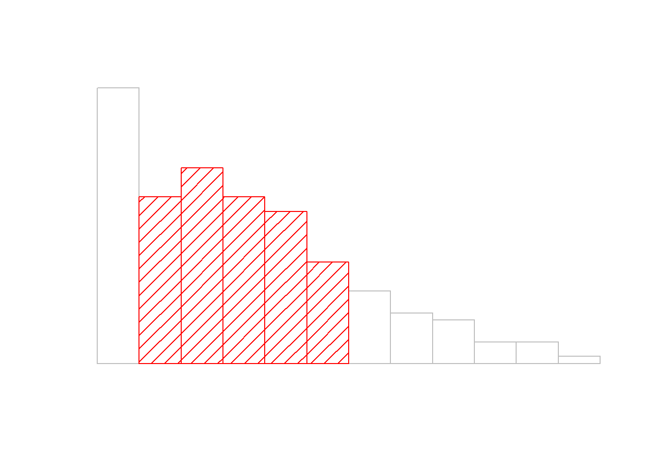
# mean absolute deviation from the mean:
mean( abs(afl.margins - mean(afl.margins)) )


#
## [1] 21.10124
## [1] 19.5
The median winning margin in 2010 was 30.5, indicating that a typical game involved a winning margin of about 30 points. However, there was a fair amount of variation from game to game: the MAD value was 19.5, indicating that a typical winning margin would differ from this median value by about 19-20 points.
mad(). However, it’s a little bit more complicated than the functions that we’ve been using previously. If you want to use it to calculate MAD in the exact same way that I have described it above, the command that you need to use specifies two arguments: the data set itself x, and a constant that I’ll explain in a moment. For our purposes, the constant is 1, so our command becomes
mad( x = afl.margins, constant = 1 )
## [1] 19.5
constant = 1 part, this is pretty straightforward.
constant = 1 argument? I won’t go into all the details here, but here’s the gist. Although the "raw" MAD value that I’ve described above is completely interpretable on its own terms, that’s not actually how it’s used in a lot of real world contexts. Instead, what happens a lot is that the researcher actually wants to calculate the standard deviation. However, in the same way that the mean is very sensitive to extreme values, the standard deviation is vulnerable to the exact same issue. So, in much the same way that people sometimes use the median as a "robust" way of calculating "something that is like the mean", it’s not uncommon to use MAD as a method for calculating "something that is like the standard deviation". Unfortunately, the raw MAD value doesn’t do this. Our raw MAD value is 19.5, and our standard deviation was 26.07. However, what some clever person has shown is that, under certain assumptionsconstant is 1.4826, and so when you use the mad() command without manually setting a value, here’s what you get:
mad( afl.margins )
## [1] 28.9107
afl.margins data, so in this case I wouldn’t try to use the MAD value this way.
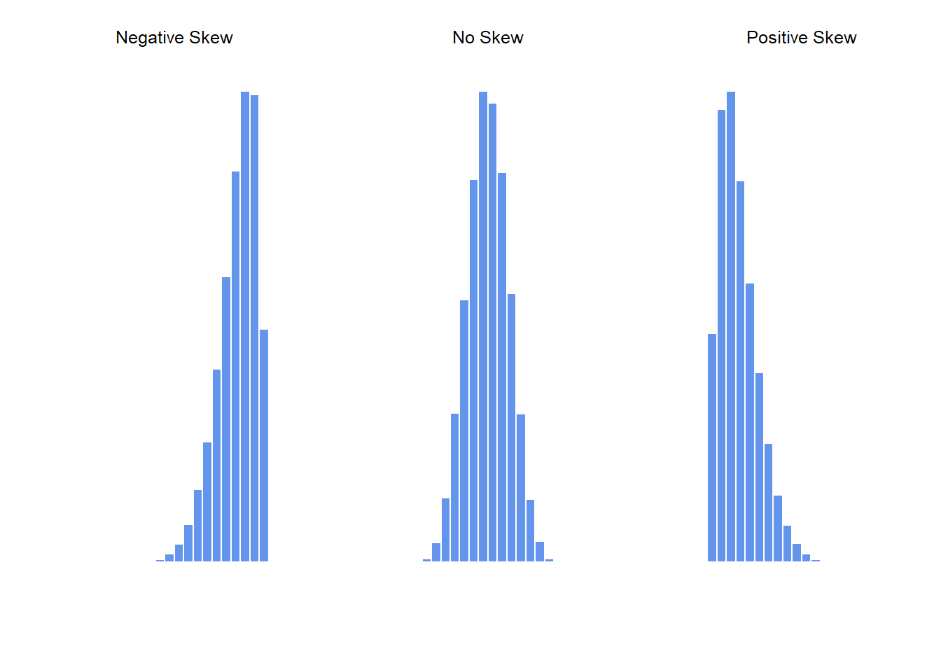
psych package contains a skew() function that you can use to calculate skewness. So if we wanted to use this function to calculate the skewness of the afl.margins data, we’d first need to load the packagelibrary( psych )
skew( x = afl.margins )
## [1] 0.7671555
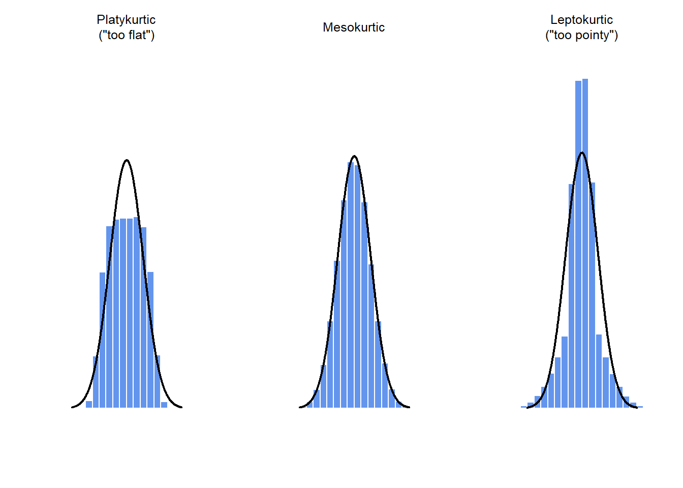
| informal term | technical name | kurtosis value |
|---|---|---|
| too flat | platykurtic | negative |
| just pointy enough | mesokurtic | zero |
| too pointy | leptokurtic | positive |
psych package has a function called kurtosi() that you can use to calculate the kurtosis of your data. For instance, if we were to do this for the AFL margins,kurtosi( x = afl.margins )
## [1] 0.02962633
summary() or describe(), perhaps? Why yes, yes it would. So much so that both of these functions exist. The summary() function is in the base package, so it comes with every installation of R. The describe() function is part of the psych package, which we loaded earlier in the chapter.
summary() function is an easy thing to use, but a tricky thing to understand in full, since it’s a generic function (see Section 4.11. The basic idea behind the summary() function is that it prints out some useful information about whatever object (i.e., variable, as far as we’re concerned) you specify as the object argument. As a consequence, the behaviour of the summary() function differs quite dramatically depending on the class of the object that you give it. Let’s start by giving it a numeric object:
summary( object = afl.margins )
##    Min. 1st Qu.  Median    Mean 3rd Qu.    Max.
##    0.00   12.75   30.50   35.30   50.50  116.00
blowouts in which the \(i\)-th element is TRUE if that game was a blowout according to my definition,
blowouts <-  afl.margins > 50
blowouts
##   [1]  TRUE FALSE  TRUE FALSE FALSE FALSE FALSE  TRUE FALSE FALSE FALSE
##  [12]  TRUE FALSE FALSE  TRUE FALSE FALSE FALSE FALSE  TRUE FALSE FALSE
##  [23] FALSE FALSE FALSE FALSE FALSE  TRUE FALSE  TRUE  TRUE FALSE FALSE
##  [34]  TRUE FALSE FALSE  TRUE FALSE FALSE FALSE FALSE FALSE FALSE FALSE
##  [45] FALSE  TRUE  TRUE FALSE FALSE FALSE FALSE FALSE  TRUE  TRUE FALSE
##  [56]  TRUE FALSE FALSE FALSE FALSE  TRUE FALSE FALSE FALSE FALSE FALSE
##  [67]  TRUE FALSE FALSE FALSE FALSE FALSE FALSE  TRUE FALSE FALSE FALSE
##  [78] FALSE FALSE  TRUE FALSE FALSE FALSE FALSE FALSE FALSE FALSE FALSE
##  [89] FALSE FALSE  TRUE FALSE FALSE  TRUE FALSE FALSE FALSE FALSE FALSE
## [100] FALSE  TRUE FALSE FALSE FALSE  TRUE FALSE  TRUE  TRUE  TRUE FALSE
## [111] FALSE FALSE FALSE FALSE FALSE FALSE FALSE FALSE FALSE  TRUE FALSE
## [122]  TRUE FALSE FALSE FALSE FALSE FALSE FALSE FALSE  TRUE  TRUE FALSE
## [133] FALSE  TRUE  TRUE FALSE FALSE FALSE FALSE FALSE  TRUE FALSE  TRUE
## [144]  TRUE  TRUE  TRUE FALSE FALSE FALSE  TRUE FALSE FALSE  TRUE FALSE
## [155]  TRUE FALSE  TRUE FALSE FALSE  TRUE FALSE FALSE  TRUE FALSE FALSE
## [166] FALSE FALSE FALSE FALSE FALSE FALSE FALSE FALSE FALSE FALSE FALSE
summary( object = blowouts )
##    Mode   FALSE    TRUE
## logical     132      44
summary() function gives us a count of the number of TRUE values, the number of FALSE values, and the number of missing values (i.e., the NAs). Pretty reasonable behaviour.
afl.finalists vector as a factor, so let’s use that:
summary( object = afl.finalists )
##         Adelaide         Brisbane          Carlton      Collingwood
##               26               25               26               28
##         Essendon          Fitzroy        Fremantle          Geelong
##               32                0                6               39
##         Hawthorn        Melbourne  North Melbourne    Port Adelaide
##               27               28               28               17
##         Richmond         St Kilda           Sydney       West Coast
##                6               24               26               38
## Western Bulldogs
##               24
table() function. Interestingly, however, if we convert this to a character vector using the as.character() function (see Section 7.10, we don’t get the same results:
f2 <- as.character( afl.finalists )
summary( object = f2 )
##    Length     Class      Mode
##       400 character character
afl.finalists as a factor, R knows that it should treat it as a nominal scale variable, and so it gives you a much more detailed (and helpful) summary than it would have if I’d left it as a character vector.
summary() function, it produces a slightly condensed summary of each variable inside the data frame. To give you a sense of how this can be useful, let’s try this for a new data set, one that you’ve never seen before. The data is stored in the clinicaltrial.Rdata file, and we’ll use it a lot in Chapter 14 (you can find a complete description of the data at the start of that chapter). Let’s load it, and see what we’ve got:
load( "./data/clinicaltrial.Rdata" )
who(TRUE)
##    -- Name --    -- Class --   -- Size --
##    clin.trial    data.frame    18 x 3
##     $drug        factor        18
##     $therapy     factor        18
##     $mood.gain   numeric       18
clin.trial which contains three variables, drug, therapy and mood.gain. Presumably then, this data is from a clinical trial of some kind, in which people were administered different drugs; and the researchers looked to see what the drugs did to their mood. Let’s see if the summary() function sheds a little more light on this situation:
summary( clin.trial )
##        drug         therapy    mood.gain
##  placebo :6   no.therapy:9   Min.   :0.1000
##  anxifree:6   CBT       :9   1st Qu.:0.4250
##  joyzepam:6                  Median :0.8500
##                              Mean   :0.8833
##                              3rd Qu.:1.3000
##                              Max.   :1.8000
mood.gain variable that most people did show a mood gain (mean \(=.88\)), though without knowing what the scale is here it’s hard to say much more than that. Still, that’s not too bad. Overall, I feel that I learned something from that.
describe() function (in the psych package) is a little different, and it’s really only intended to be useful when your data are interval or ratio scale. Unlike the summary() function, it calculates the same descriptive statistics for any type of variable you give it. By default, these are:
var. This is just an index: 1 for the first variable, 2 for the second variable, and so on.
n. This is the sample size: more precisely, it’s the number of non-missing values.
min. The minimum value.
max. The maximum value.
describe() function does is convert factors and logical variables to numeric vectors in order to do the calculations. These variables are marked with * and most of the time, the descriptive statistics for those variables won’t make much sense. If you try to feed it a data frame that includes a character vector as a variable, it produces an error.
describe() function to have a look at the clin.trial data frame. Here’s what we get:
describe( x = clin.trial )
##           vars  n mean   sd median trimmed  mad min max range skew
## drug*        1 18 2.00 0.84   2.00    2.00 1.48 1.0 3.0   2.0 0.00
## therapy*     2 18 1.50 0.51   1.50    1.50 0.74 1.0 2.0   1.0 0.00
## mood.gain    3 18 0.88 0.53   0.85    0.88 0.67 0.1 1.8   1.7 0.13
##           kurtosis   se
## drug*        -1.66 0.20
## therapy*     -2.11 0.12
## mood.gain    -1.44 0.13
mood.gain variable, there’s a lot of useful information.
by(), describeBy() and aggregate(). Let’s start with the describeBy() function, which is part of the psych package. The describeBy() function is very similar to the describe() function, except that it has an additional argument called group which specifies a grouping variable. For instance, let’s say, I want to look at the descriptive statistics for the clin.trial data, broken down separately by therapy type. The command I would use here is:
describeBy( x=clin.trial, group=clin.trial$therapy )
##
##  Descriptive statistics by group
## group: no.therapy
##           vars n mean   sd median trimmed  mad min max range skew kurtosis
## drug*        1 9 2.00 0.87    2.0    2.00 1.48 1.0 3.0   2.0 0.00    -1.81
## therapy*     2 9 1.00 0.00    1.0    1.00 0.00 1.0 1.0   0.0  NaN      NaN
## mood.gain    3 9 0.72 0.59    0.5    0.72 0.44 0.1 1.7   1.6 0.51    -1.59
##             se
## drug*     0.29
## therapy*  0.00
## mood.gain 0.20
## --------------------------------------------------------
## group: CBT
##           vars n mean   sd median trimmed  mad min max range  skew
## drug*        1 9 2.00 0.87    2.0    2.00 1.48 1.0 3.0   2.0  0.00
## therapy*     2 9 2.00 0.00    2.0    2.00 0.00 2.0 2.0   0.0   NaN
## mood.gain    3 9 1.04 0.45    1.1    1.04 0.44 0.3 1.8   1.5 -0.03
##           kurtosis   se
## drug*        -1.81 0.29
## therapy*       NaN 0.00
## mood.gain    -1.12 0.15
describe() function produce, except that the output now gives you means, standard deviations etc separately for the CBT group and the no.therapy group. Notice that, as before, the output displays asterisks for factor variables, in order to draw your attention to the fact that the descriptive statistics that it has calculated won’t be very meaningful for those variables. Nevertheless, this command has given us some really useful descriptive statistics mood.gain variable, broken down as a function of therapy.
by() function. There are three arguments that you need to specify when using this function: the data argument specifies the data set, the INDICES argument specifies the grouping variable, and the FUN argument specifies the name of a function that you want to apply separately to each group. To give a sense of how powerful this is, you can reproduce the describeBy() function by using a command like this:
by( data=clin.trial, INDICES=clin.trial$therapy, FUN=describe )
describe() function. You could just as easily use the by() function in conjunction with the summary() function. For example:
by( data=clin.trial, INDICES=clin.trial$therapy, FUN=summary )
## clin.trial$therapy: no.therapy
##        drug         therapy    mood.gain
##  placebo :3   no.therapy:9   Min.   :0.1000
##  anxifree:3   CBT       :0   1st Qu.:0.3000
##  joyzepam:3                  Median :0.5000
##                              Mean   :0.7222
##                              3rd Qu.:1.3000
##                              Max.   :1.7000
## --------------------------------------------------------
## clin.trial$therapy: CBT
##        drug         therapy    mood.gain
##  placebo :3   no.therapy:0   Min.   :0.300
##  anxifree:3   CBT       :9   1st Qu.:0.800
##  joyzepam:3                  Median :1.100
##                              Mean   :1.044
##                              3rd Qu.:1.300
##                              Max.   :1.800
summary() function, applied separately to CBT group and the no.therapy group. For the two factors (drug and therapy) it prints out a frequency table, whereas for the numeric variable (mood.gain) it prints out the range, interquartile range, mean and median.
by() and describeBy() functions, but I usually find it more convenient to use the aggregate() function in this situation. There are again three arguments that you need to specify. The formula argument is used to indicate which variable you want to analyse, and which variables are used to specify the groups. For instance, if you want to look at mood.gain separately for each possible combination of drug and therapy, the formula you want is mood.gain ~ drug + therapy. The data argument is used to specify the data frame containing all the data, and the FUN argument is used to indicate what function you want to calculate for each group (e.g., the mean). So, to obtain group means, use this command:
aggregate( formula = mood.gain ~ drug + therapy,  # mood.gain by drug/therapy combination
           data = clin.trial,                     # data is in the clin.trial data frame
           FUN = mean                             # print out group means
)
##       drug    therapy mood.gain
## 1  placebo no.therapy  0.300000
## 2 anxifree no.therapy  0.400000
## 3 joyzepam no.therapy  1.466667
## 4  placebo        CBT  0.600000
## 5 anxifree        CBT  1.033333
## 6 joyzepam        CBT  1.500000
aggregate( mood.gain ~ drug + therapy, clin.trial, sd )
##       drug    therapy mood.gain
## 1  placebo no.therapy 0.2000000
## 2 anxifree no.therapy 0.2000000
## 3 joyzepam no.therapy 0.2081666
## 4  placebo        CBT 0.3000000
## 5 anxifree        CBT 0.2081666
## 6 joyzepam        CBT 0.2645751
X, the simplest way is to use a command like (X - mean(X)) / sd(X). There’s also a fancier function called scale() that you can use, but it relies on somewhat more complicated R concepts that I haven’t explained yet.
pnorm() that allows us to be a bit more precise than this. Specifically, it allows us to calculate a theoretical percentile rank for my grumpiness, as follows:pnorm( 3.6 )
## [1] 0.9998409
parenthood.Rdata. If we load the data...
load( "./data/parenthood.Rdata" )
who(TRUE)
##    -- Name --     -- Class --   -- Size --
##    parenthood     data.frame    100 x 4
##     $dan.sleep    numeric       100
##     $baby.sleep   numeric       100
##     $dan.grump    numeric       100
##     $day          integer       100
parenthood, which contains four variables dan.sleep, baby.sleep, dan.grump and day. If we peek at the data using head() out the data, here’s what we get:
head(parenthood,10)
##    dan.sleep baby.sleep dan.grump day
## 1       7.59      10.18        56   1
## 2       7.91      11.66        60   2
## 3       5.14       7.92        82   3
## 4       7.71       9.61        55   4
## 5       6.68       9.75        67   5
## 6       5.99       5.04        72   6
## 7       8.19      10.45        53   7
## 8       7.19       8.27        60   8
## 9       7.40       6.06        60   9
## 10      6.58       7.09        71  10
describe( parenthood )
##            vars   n  mean    sd median trimmed   mad   min    max range
## dan.sleep     1 100  6.97  1.02   7.03    7.00  1.09  4.84   9.00  4.16
## baby.sleep    2 100  8.05  2.07   7.95    8.05  2.33  3.25  12.07  8.82
## dan.grump     3 100 63.71 10.05  62.00   63.16  9.64 41.00  91.00 50.00
## day           4 100 50.50 29.01  50.50   50.50 37.06  1.00 100.00 99.00
##             skew kurtosis   se
## dan.sleep  -0.29    -0.72 0.10
## baby.sleep -0.02    -0.69 0.21
## dan.grump   0.43    -0.16 1.00
## day         0.00    -1.24 2.90
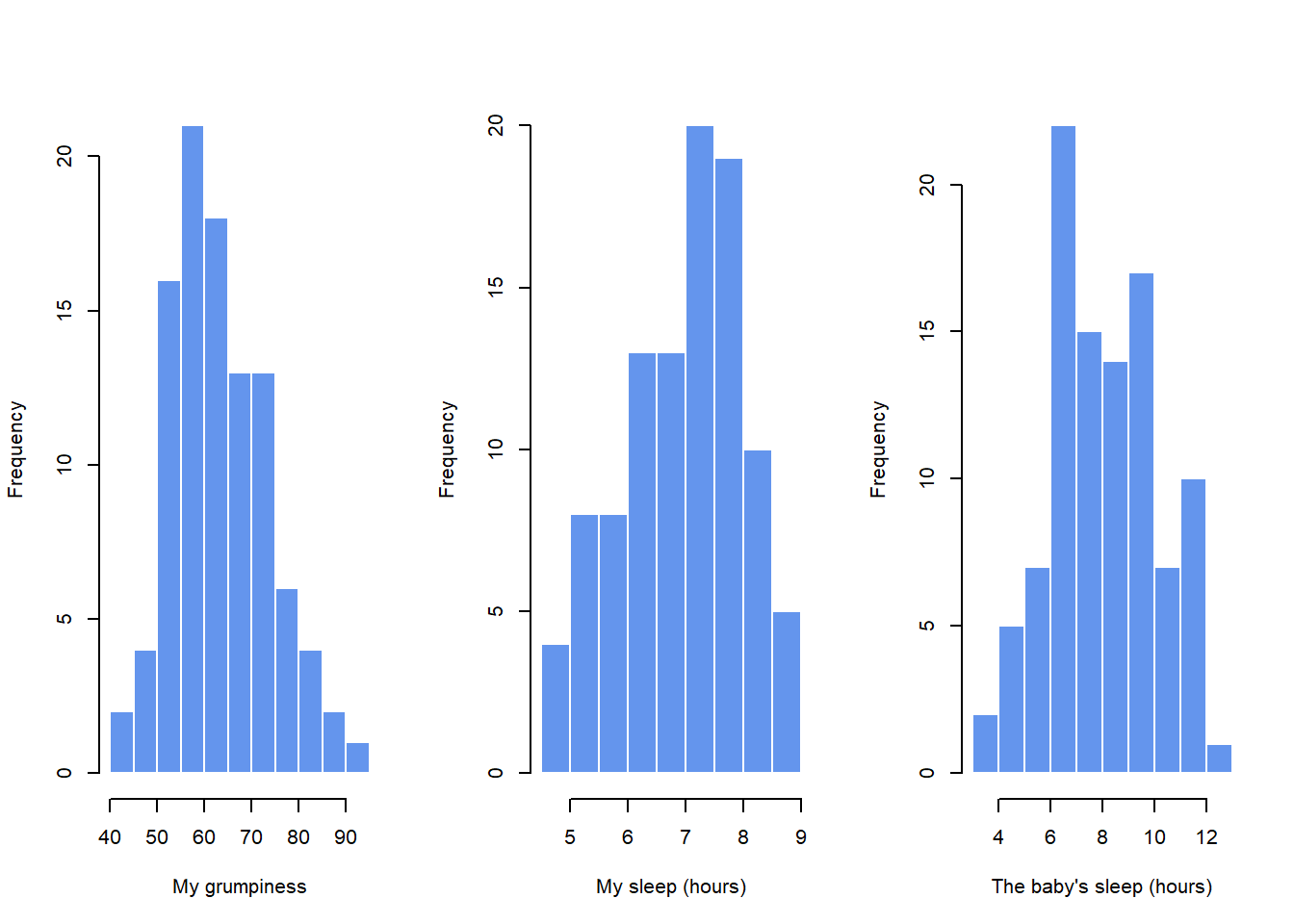
parenthood data set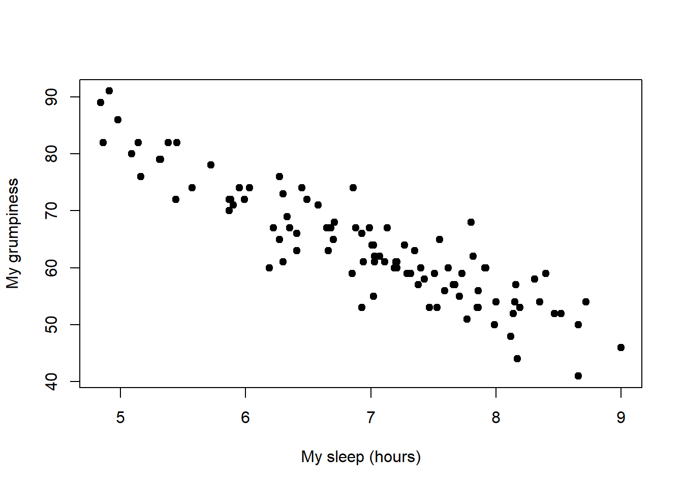
dan.sleep and dan.grump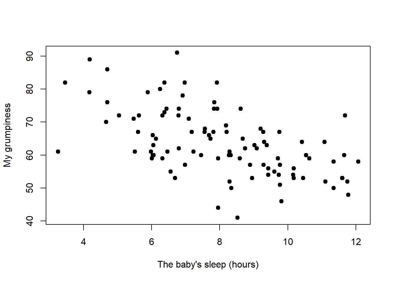
baby.sleep and dan.grumpdan.sleep and dan.grump (Figure 5.67 with that between baby.sleep and dan.grump (Figure 5.68. When looking at these two plots side by side, it’s clear that the relationship is qualitatively the same in both cases: more sleep equals less grump! However, it’s also pretty obvious that the relationship between dan.sleep and dan.grump is stronger than the relationship between baby.sleep and dan.grump. The plot on the left is "neater" than the one on the right. What it feels like is that if you want to predict what my mood is, it’d help you a little bit to know how many hours my son slept, but it’d be more helpful to know how many hours I slept.
baby.sleep v dan.grump" to the scatterplot of "baby.sleep v dan.sleep", the overall strength of the relationship is the same, but the direction is different. That is, if my son sleeps more, I get more sleep (positive relationship, but if he sleeps more then I get less grumpy (negative relationship).
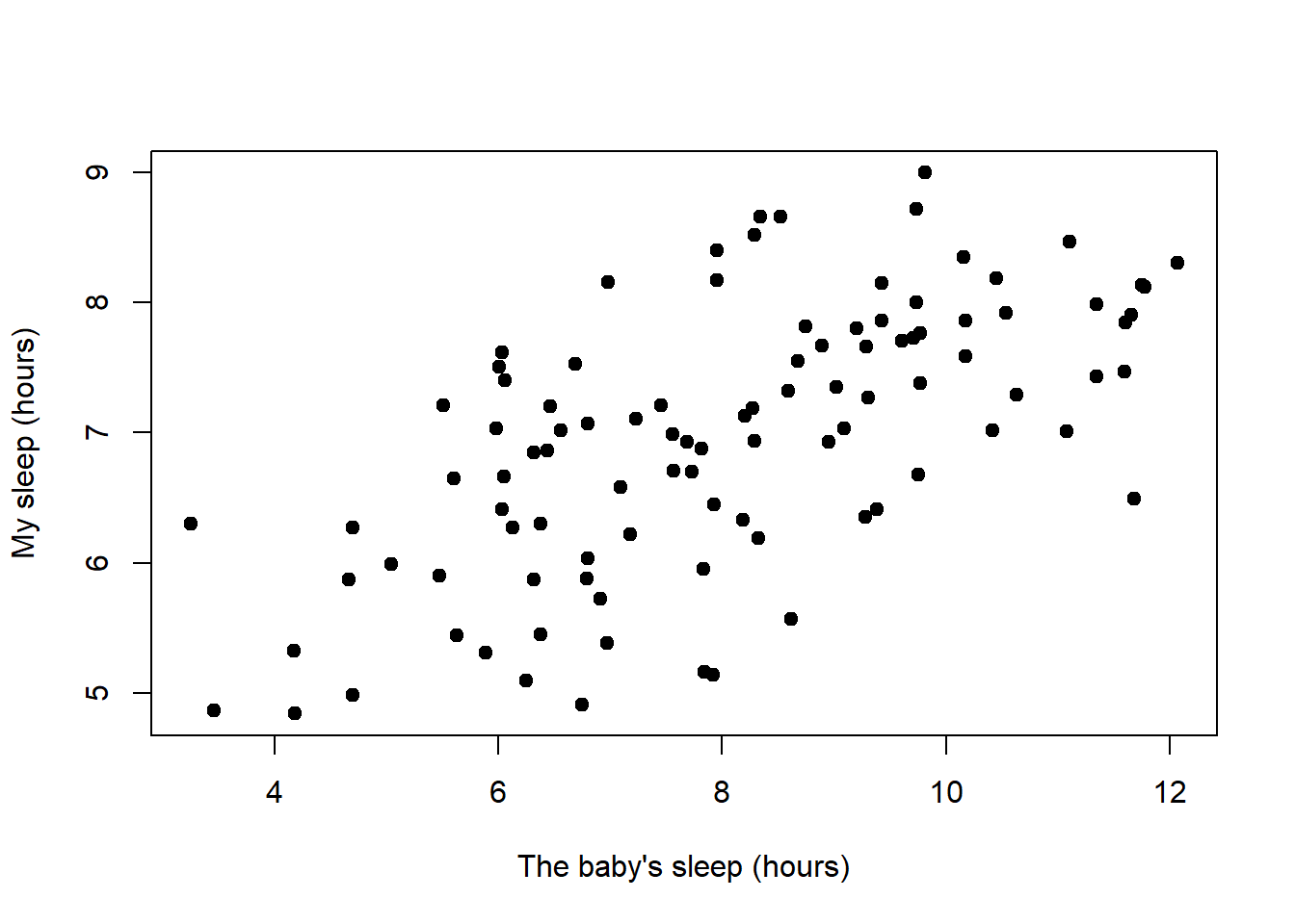
baby.sleep and dan.sleep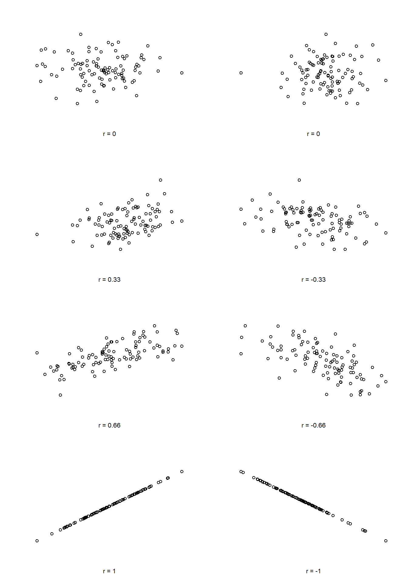
dan.sleep variable (units: hours) and \(Y\) refers to the dan.grump variable (units: grumps), then the units for their covariance are "hours \(\times\) grumps". And I have no freaking idea what that would even mean.cor() command. The simplest way to use the command is to specify two input arguments x and y, each one corresponding to one of the variables. The following extract illustrates the basic usage of the function:cor.test() that runs a hypothesis test for a single correlation, and the psych package contains a version called corr.test() that can run tests for every correlation in a correlation matrix; hypothesis tests for correlations are discussed in more detail in Section 15.6.
cor( x = parenthood$dan.sleep, y = parenthood$dan.grump )
## [1] -0.903384
cor() function is a bit more powerful than this simple example suggests. For example, you can also calculate a complete "correlation matrix", between all pairs of variables in the data frame:cor() is to correlate one set of variables with another subset of variables. If X and Y are both data frames with the same number of rows, then cor(x = X, y = Y) will produce a correlation matrix that correlates all variables in X with all variables in Y.
# correlate all pairs of variables in "parenthood":
cor( x = parenthood )
##              dan.sleep  baby.sleep   dan.grump         day
## dan.sleep   1.00000000  0.62794934 -0.90338404 -0.09840768
## baby.sleep  0.62794934  1.00000000 -0.56596373 -0.01043394
## dan.grump  -0.90338404 -0.56596373  1.00000000  0.07647926
## day        -0.09840768 -0.01043394  0.07647926  1.00000000
| Correlation | Strength | Direction |
|---|---|---|
| -1.0 to -0.9 | Very strong | Negative |
| -0.9 to -0.7 | Strong | Negative |
| -0.7 to -0.4 | Moderate | Negative |
| -0.4 to -0.2 | Weak | Negative |
| -0.2 to 0 | Negligible | Negative |
| 0 to 0.2 | Negligible | Positive |
| 0.2 to 0.4 | Weak | Positive |
| 0.4 to 0.7 | Moderate | Positive |
| 0.7 to 0.9 | Strong | Positive |
| 0.9 to 1.0 | Very strong | Positive |
cor( anscombe$x1, anscombe$y1 )
cor( anscombe$x2, anscombe$y2 )
## [1] 0.8164205
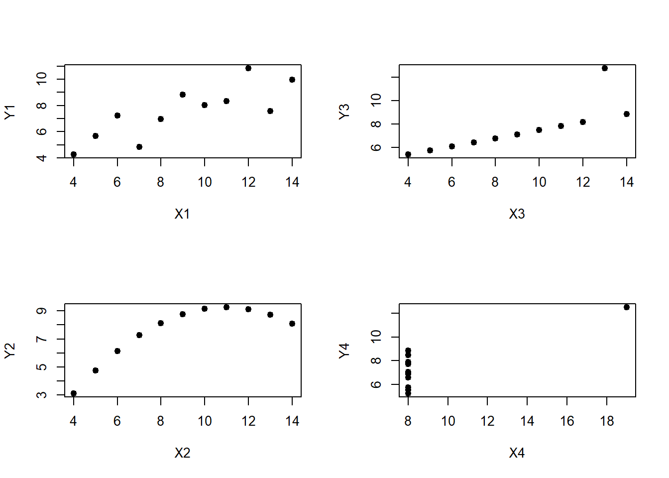
effort.Rdata:
> load( "effort.Rdata" )
> who(TRUE)
   -- Name --   -- Class --   -- Size --
   effort       data.frame    10 x 2
    $hours      numeric       10
    $grade      numeric       10
> effort
   hours grade
1      2    13
2     76    91
3     40    79
4      6    14
5     16    21
6     28    74
7     27    47
8     59    85
9     46    84
10    68    88
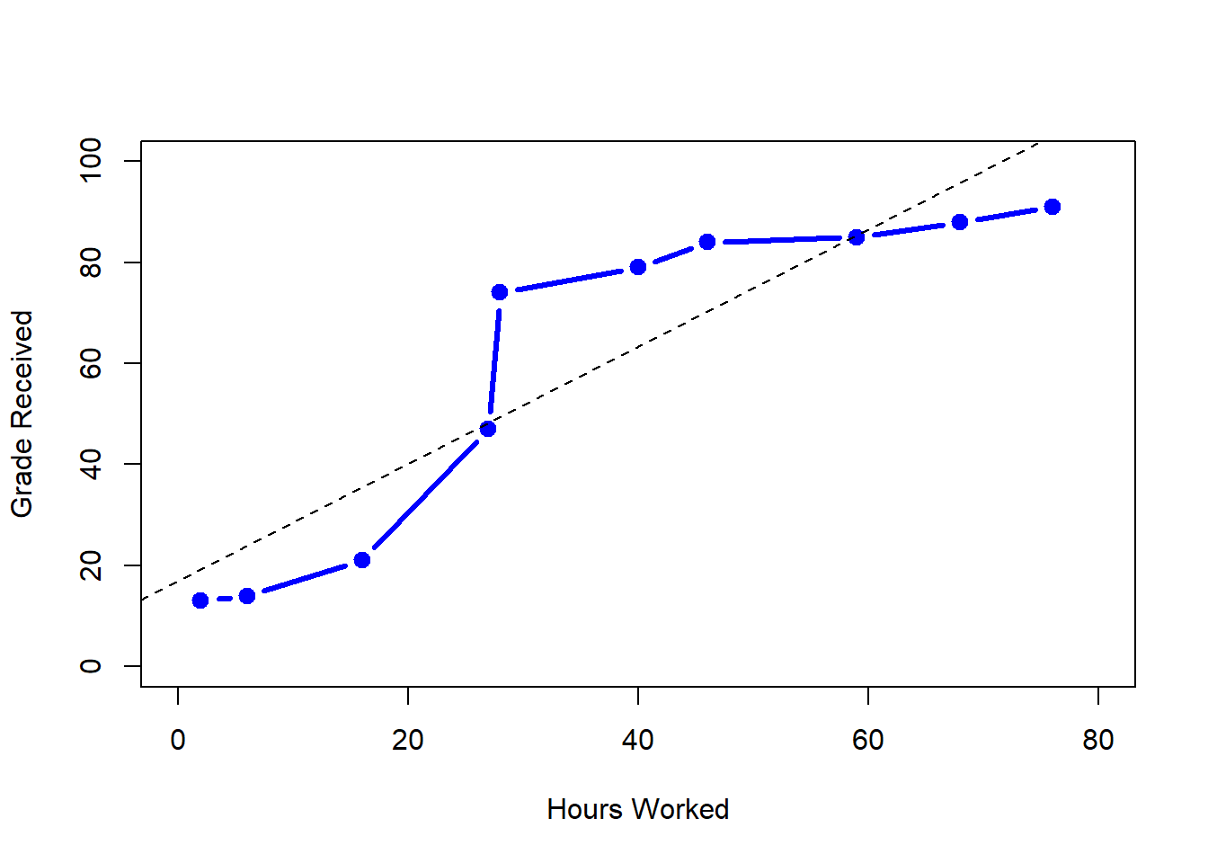
> cor( effort$hours, effort$grade )
[1] 0.909402
| student | rank (hours worked) | rank (grade received) |
|---|---|---|
| student 1 | 1 | 1 |
| student 2 | 10 | 10 |
| student 3 | 6 | 6 |
| student 4 | 2 | 2 |
| student 5 | 3 | 3 |
| student 6 | 5 | 5 |
| student 7 | 4 | 4 |
| student 8 | 8 | 8 |
| student 9 | 7 | 7 |
| student 10 | 9 | 9 |
rank() function, like this:
> hours.rank <- rank( effort$hours )   # rank students by hours worked
> grade.rank <- rank( effort$grade )   # rank students by grade received
> cor( hours.rank, grade.rank )
[1] 1
rank() function to construct the rankings, and then calculate the Pearson correlation on these ranks. However, that’s way too much effort to do every time. It’s much easier to just specify the method argument of the cor() function.
> cor( effort$hours, effort$grade, method = "spearman")
[1] 1
method argument is "pearson", which is why we didn’t have to specify it earlier on when we were doing Pearson correlations.
correlate() function
cor() function works pretty well, and handles many of the situations that you might be interested in. One thing that many beginners find frustrating, however, is the fact that it’s not built to handle non-numeric variables. From a statistical perspective, this is perfectly sensible: Pearson and Spearman correlations are only designed to work for numeric variables, so the cor() function spits out an error.
hours you worked in any given day, and counted how many tasks you completed. If you were doing the tasks for money, you might also want to keep track of how much pay you got for each job. It would also be sensible to keep track of the weekday on which you actually did the work: most of us don’t work as much on Saturdays or Sundays. If you did this for 7 weeks, you might end up with a data set that looks like this one:
> load("work.Rdata")

> who(TRUE)
   -- Name --   -- Class --   -- Size --
   work         data.frame    49 x 7
    $hours      numeric       49
    $tasks      numeric       49
    $pay        numeric       49
    $day        integer       49
    $weekday    factor        49
    $week       numeric       49
    $day.type   factor        49

> head(work)
  hours tasks pay day   weekday week day.type
1   7.2    14  41   1   Tuesday    1  weekday
2   7.4    11  39   2 Wednesday    1  weekday
3   6.6    14  13   3  Thursday    1  weekday
4   6.5    22  47   4    Friday    1  weekday
5   3.1     5   4   5  Saturday    1  weekend
6   3.0     7  12   6    Sunday    1  weekend
hours with pay quite using cor(), like so:
> cor(work$hours,work$pay)
[1] 0.7604283
work data frame, because it contains two factor variables, weekday and day.type. If I try this, I get an error:
> cor(work)
Error in cor(work) : 'x' must be numeric
cor() function, is create a new data frame that doesn’t contain the factor variables, and then feed that new data frame into the cor() function. It’s not actually very hard to do that, and I’ll talk about how to do it properly in Section 7.5. But it would be nice to have some function that is smart enough to just ignore the factor variables. That’s where the correlate() function in the lsr package can be handy. If you feed it a data frame that contains factors, it knows to ignore them, and returns the pairwise correlations only between the numeric variables:
> correlate(work)

CORRELATIONS
============
- correlation type:  pearson
- correlations shown only when both variables are numeric

          hours  tasks   pay    day weekday   week day.type
hours         .  0.800 0.760 -0.049       .  0.018        .
tasks     0.800      . 0.720 -0.072       . -0.013        .
pay       0.760  0.720     .  0.137       .  0.196        .
day      -0.049 -0.072 0.137      .       .  0.990        .
weekday       .      .     .      .       .      .        .
week      0.018 -0.013 0.196  0.990       .      .        .
day.type      .      .     .      .       .      .        .
. whenever one of the variables is non-numeric. It also shows a . whenever a variable is correlated with itself (it’s not a meaningful thing to do). The correlate() function can also do Spearman correlations, by specifying the corr.method to use:
> correlate( work, corr.method="spearman" )

CORRELATIONS
============
- correlation type:  spearman
- correlations shown only when both variables are numeric

          hours  tasks   pay    day weekday   week day.type
hours         .  0.805 0.745 -0.047       .  0.010        .
tasks     0.805      . 0.730 -0.068       . -0.008        .
pay       0.745  0.730     .  0.094       .  0.154        .
day      -0.047 -0.068 0.094      .       .  0.990        .
weekday       .      .     .      .       .      .        .
week      0.010 -0.008 0.154  0.990       .      .        .
day.type      .      .     .      .       .      .        .
correlate() function, and any advanced R user would be perfectly capable of using the cor() function to get these numbers out. But if you’re not yet comfortable with extracting a subset of a data frame, the correlate() function is for you.
NA values in your data vector. Let’s create a variable like that:
> partial <- c(10, 20, NA, 30)
NA is "I don’t know what this number is". This means that 1 + NA = NA: if I add 1 to some number that I don’t know (i.e., the NA) then the answer is also a number that I don’t know. As a consequence, if you don’t explicitly tell R to ignore the NA values, and the data set does have missing values, then the output will itself be a missing value. If I try to calculate the mean of the partial vector, without doing anything about the missing value, here’s what happens:
> mean( x = partial )
[1] NA
cor() which is a special case I’ll discuss below) have an optional argument called na.rm, which is shorthand for "remove NA values". By default, na.rm = FALSE, so R does nothing about the missing data problem. Let’s try setting na.rm = TRUE and see what happens:
NA values) there’s actually an additional argument to the function that you should be aware of. This argument is called na.rm, and is a logical value indicating whether R should ignore (or "remove") the missing data for the purposes of doing the calculations. By default, R assumes that you want to keep the missing values, so unless you say otherwise it will set na.rm = FALSE. However, R assumes that 1 + NA = NA: if I add 1 to some number that I don’t know (i.e., the NA) then the answer is also a number that I don’t know. As a consequence, if you don’t explicitly tell R to ignore the NA values, and the data set does have missing values, then the output will itself be a missing value. This is illustrated in the following extract:
> mean( x = partial, na.rm = TRUE )
[1] 20
20 (i.e., 60 / 3) and not 15. When R ignores a NA value, it genuinely ignores it. In effect, the calculation above is identical to what you’d get if you asked for the mean of the three-element vector c(10, 20, 30).
mean() function. Pretty much all of the other functions that I’ve talked about in this chapter have an na.rm argument that indicates whether it should ignore missing values. However, its behaviour is the same for all these functions, so I won’t waste everyone’s time by demonstrating it separately for each one.
cor() function is a special case. It doesn’t have an na.rm argument, because the story becomes a lot more complicated when more than one variable is involved. What it does have is an argument called use which does roughly the same thing, but you need to think little more carefully about what you want this time. To illustrate the issues, let’s open up a data set that has missing values, parenthood2.Rdata. This file contains the same data as the original parenthood data, but with some values deleted. It contains a single data frame, parenthood2:
> load( "parenthood2.Rdata" )
> print( parenthood2 )
  dan.sleep baby.sleep dan.grump day
1      7.59         NA        56   1
2      7.91      11.66        60   2
3      5.14       7.92        82   3
4      7.71       9.61        55   4
5      6.68       9.75        NA   5
6      5.99       5.04        72   6
BLAH BLAH BLAH
describe() function
> describe( parenthood2 )
           var   n  mean    sd median trimmed   mad   min    max    BLAH
dan.sleep    1  91  6.98  1.02   7.03    7.02  1.13  4.84   9.00    BLAH
baby.sleep   2  89  8.11  2.05   8.20    8.13  2.28  3.25  12.07    BLAH
dan.grump    3  92 63.15  9.85  61.00   62.66 10.38 41.00  89.00    BLAH
day          4 100 50.50 29.01  50.50   50.50 37.06  1.00 100.00    BLAH
n column that there are 9 missing values for dan.sleep, 11 missing values for baby.sleep and 8 missing values for dan.grump.NA values. This is because, while describe() also has an na.rm argument, the default value for this function is na.rm = TRUE.
> cor( parenthood2 )
           dan.sleep baby.sleep dan.grump day
dan.sleep          1         NA        NA  NA
baby.sleep        NA          1        NA  NA
dan.grump         NA         NA         1  NA
day               NA         NA        NA   1
dan.sleep and baby.sleep actually are, then I can’t possibly know what the correlation between these two variables is either, since the formula for the correlation coefficient makes use of every single observation in the data set. Once again, it makes sense: it’s just not particularly helpful.
use argument to the cor() function. There are several different values that you can specify for this, but the two that we care most about in practice tend to be "complete.obs" and "pairwise.complete.obs". If we specify use = "complete.obs", R will completely ignore all cases (i.e., all rows in our parenthood2 data frame) that have any missing values at all. So, for instance, if you look back at the extract earlier when I used the head() function, notice that observation 1 (i.e., day 1) of the parenthood2 data set is missing the value for baby.sleep, but is otherwise complete? Well, if you choose use = "complete.obs" R will ignore that row completely: that is, even when it’s trying to calculate the correlation between dan.sleep and dan.grump, observation 1 will be ignored, because the value of baby.sleep is missing for that observation. Here’s what we get:
> cor(parenthood2, use = "complete.obs")
             dan.sleep baby.sleep   dan.grump         day
dan.sleep   1.00000000  0.6394985 -0.89951468  0.06132891
baby.sleep  0.63949845  1.0000000 -0.58656066  0.14555814
dan.grump  -0.89951468 -0.5865607  1.00000000 -0.06816586
day         0.06132891  0.1455581 -0.06816586  1.00000000
use = "pairwise.complete.obs". When we do that, R only looks at the variables that it’s trying to correlate when determining what to drop. So, for instance, since the only missing value for observation 1 of parenthood2 is for baby.sleep R will only drop observation 1 when baby.sleep is one of the variables involved: and so R keeps observation 1 when trying to correlate dan.sleep and dan.grump. When we do it this way, here’s what we get:
> cor(parenthood2, use = "pairwise.complete.obs")
             dan.sleep  baby.sleep    dan.grump          day
dan.sleep   1.00000000  0.61472303 -0.903442442 -0.076796665
baby.sleep  0.61472303  1.00000000 -0.567802669  0.058309485
dan.grump  -0.90344244 -0.56780267  1.000000000  0.005833399
day        -0.07679667  0.05830949  0.005833399  1.000000000
correlate() function (in the lsr package) automatically uses the "pairwise complete" method:
> correlate(parenthood2)

CORRELATIONS
============
- correlation type:  pearson
- correlations shown only when both variables are numeric

           dan.sleep baby.sleep dan.grump    day
dan.sleep          .      0.615    -0.903 -0.077
baby.sleep     0.615          .    -0.568  0.058
dan.grump     -0.903     -0.568         .  0.006
day           -0.077      0.058     0.006      .
The death of one man is a tragedy. The death of millions is a statistic. — Josef Stalin, Potsdam 1945
| Variable | Min | Max | Mean | Median | Std. Dev | IQR |
|---|---|---|---|---|---|---|
| Dan’s grumpiness | 41 | 91 | 63.71 | 62 | 10.05 | 14 |
| Dan’s hours slept | 4.84 | 9.00 | 6.97 | 7.03 | 1.02 | 1.45 |
| Dan’s son’s hours slept | 3.25 | 12.07 | 8.05 | 7.95 | 2.07 | 3.21 |

