Linear Regression

Chapter 3 Linear Regression

Quick review of equations for lines:

Recall the equation of a line is usually in the form $y=mx+b\text{,}$ where $x$ and $y$ are variables and $m$ and $b$ are numbers. Some basic facts about lines:

🔗

If you are given a number for $x\text{,}$ you can plug it in to the equation $y=mx+b$ to get a number for $y\text{,}$ which together give you a point with coordinates $(x,y)$ that is on the line.
🔗

🔗
$m$ is the slope, which tells how much the line goes up (increasing $y$) for every unit you move over to the right (increasing $x$) — we often say that the value of the slope is $m=\frac{rise}{run}$. The slope can be:
🔗
- positive, if the line is tilted up,
  🔗
  
  🔗
- negative, if the line is tilted down,
  🔗
  
  🔗
- zero, if the line is horizontal, and
  🔗
  
  🔗
- undefined, if the line is vertical.
  🔗
  
  🔗
🔗
You can calculate the slope by finding the coordinates $(x_1,y_1)$ and $(x_2,y_2)$ of any two points on the line and then $m=\frac{y_2-y_1}{x_2-x_1}\text{.}$
🔗

🔗
In particular, if $x_2-x_1=1\text{,}$ then $m=\frac{y_2-y_1}{1}=y_2-y_1$ — so if you look at how much the line goes up in each step of one unit to the right, that number will be the slope $m$ (and if it goes down, the slope $m$ will simply be negative). In other words, the slope answers the question “for each step to the right, how much does the line increase (or decrease)?”
🔗

🔗
$b$ is the $y$-intercept, which tells the $y$-coordinate of the point where the line crosses the $y$-axis. Another way of saying that is that $b$ is the $y$ value of the line when the $x$ is $0\text{.}$
🔗

🔗

Section 3.1 The Least Squares Regression Line

Suppose we have some bivariate quantitative data $\{(x_1,y_1), \dots , (x_n,y_n)\}$ for which the correlation coefficient indicates some linear association. It is natural to want to write down explicitly the equation of the best line through the data — the question is what is this line. The most common meaning given to best in this search for the line is the line whose total square error is the smallest possible. We make this notion precise in two steps

🔗

Definition 3.1.

Given a bivariate quantitative dataset $\{(x_1,y_1), \dots , (x_n,y_n)\}$ and a candidate line $\widehat{y}=mx+b$ passing through this dataset, a residual is the difference in $y$-coordinates of an actual data point $(x_i,y_i)$ and the line’s $y$ value at the same $x$-coordinate. That is, if the $y$-coordinate of the line when $x=x_i$ is $\widehat{y}_i=mx_i+b\text{,}$ then the residual is the measure of error given by $error_i=y_i-\widehat{y}_i\text{.}$

🔗

Note we use the convention here and elsewhere of writing $\widehat{y}$ for the $y$-coordinate on an approximating line, while the plain $y$ variable is left for actual data values, like $y_i\text{.}$

🔗

Here is an example of what residuals look like

🔗

Figure 3.2. Illustration of residuals in a scatterplot
🔗

Now we are in the position to state the

🔗

Definition 3.3.

Given a bivariate quantitative dataset the least square regression line, almost always abbreviated to LSRL, is the line for which the sum of the squares of the residuals is the smallest possible.

🔗

Fact.

If a bivariate quantitative dataset $\{(x_1,y_1), \dots , (x_n,y_n)\}$ has LSRL given by $\widehat{y}=mx+b\text{,}$ then

The slope of the LSRL is given by $m=r\frac{s_y}{s_x}\text{,}$ where $r$ is the correlation coefficient of the dataset.

🔗
The LSRL passes through the point $(\overline{x},\overline{y})$.

🔗
It follows that the $y$-intercept of the LSRL is given by $b=\overline{y}-\overline{x}\,m=\overline{y}-\overline{x}\,r\,\frac{s_y}{s_x}$.

🔗

🔗

It is possible to find the (coefficients of the) LSRL using the above information, but it is often more convenient to use a calculator or other electronic tool. Such tools also make it very easy to graph the LSRL right on top of the scatterplot — although it is often fairly easy to sketch what the LSRL will likely look like by just making a good guess, using visual intuition, if the linear association is strong (as will be indicated by the correlation coefficient).

🔗

Example 3.4.

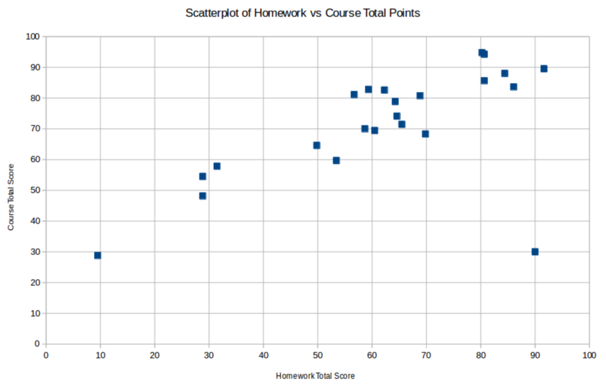
Here is some data where the individuals are 23 students in a statistics class, the independent variable is the students’ total score on their homeworks, while the dependent variable is their final total course points, both out of 100.

🔗

\begin{equation*} \begin{matrix} x:\amp 65\amp 65\amp 50\amp 53\amp 59\amp 92\amp 86\amp 84\amp 29\\ y:\amp 74\amp 71\amp 65\amp 60\amp 83\amp 90\amp 84\amp 88\amp 48\\ \ \\ x:\amp 29\amp 9\amp 64\amp 31\amp 69\amp 10\amp 57\amp 81\amp 81\\ y:\amp 54\amp 25\amp 79\amp 58\amp 81\amp 29\amp 81\amp 94\amp 86\\ \ \\ x:\amp 80\amp 70\amp 60\amp 62\amp 59\\ y:\amp 95\amp 68\amp 69\amp 83\amp 70\\ \end{matrix} \end{equation*}

Here is the resulting scatterplot, made with LibreOffice Calc (a free equivalent of Microsoft Excel)

🔗

[Figure: scatter1.eps - placeholder for scatterplot]

🔗

It seems pretty clear that there is quite a strong linear association between these two variables, as is born out by the correlation coefficient, $r=.935$ (computed with LibreOffice Calc’s CORREL). Using then STDEV.S and AVERAGE, we find that the coefficients of the LSRL for this data, $\widehat{y}=mx+b$ are

🔗

\begin{equation*} m=r\frac{s_y}{s_x}=.935\frac{18.701}{23.207}=.754\qquad{\rm and}\qquad b=\overline{y}-\overline{x}\,m=71-58\cdot .754=26.976 \end{equation*}

We can also use LibreOffice Calc’s Insert Trend Line, with Show Equation, to get all this done automatically. Note that when LibreOffice Calc writes the equation of the LSRL, it uses $f(x)$ in place of $\widehat{y}\text{,}$ as we would.

🔗

[Figure: scatter2.eps - placeholder for scatterplot with LSRL]

🔗

Section 3.2 Applications and Interpretations of LSRLs

Suppose that we have a bivariate quantitative dataset $\{(x_1,y_1), \dots , (x_n,y_n)\}$ and we have computed its correlation coefficient $r$ and (the coefficients of) its LSRL $\widehat{y}=mx+b\text{.}$ What is this information good for?

🔗

The main use of the LSRL is described in the following

🔗

Definition 3.5.

Given a bivariate quantitative dataset and associated LSRL with equation $\widehat{y}=mx+b\text{,}$ the process of guessing that the value of the dependent variable in this relationship to have the value $mx_0+b\text{,}$ for $x_0$ any value for the independent variable which satisfies $x_{min}\le x_0\le x_{max}\text{,}$ is called interpolation.

🔗

The idea of interpolation is that we think the LSRL describes as well as possible the relationship between the independent and dependent variables, so that if we have a new $x$ value, we’ll use the LSRL equation to predict what would be our best guess of what would be the corresponding $y\text{.}$ Note we might have a new value of $x$ because we simply lost part of our dataset and are trying to fill it in as best we can. Another reason might be that a new individual came along whose value of the independent variable, $x_0\text{,}$ was typical of the rest of the dataset — so the the very least $x_{min}\le x_0\le x_{max}$ — and we want to guess what will be the value of the dependent variable for this individual before we measure it. (Or maybe we cannot measure it for some reason.)

🔗

A common (but naive) alternate approach to interpolation for a value $x_0$ as above might be to find two values $x_i$ and $x_j$ in the dataset which were as close to $x_0$ as possible, and on either side of it (so $x_i\lt x_0\lt x_j$), and simply to guess that the $y$-value for $x_0$ would be the average of $y_i$ and $y_j\text{.}$ This is not a terrible idea, but it is not as effective as using the LSRL as described above, since we use the entire dataset when we build the coefficients of the LSRL. So the LSRL will give, by the process of interpolation, the best guess for what should be that missing $y$-value based on everything we know, while the “average of $y_i$ and $y_j$” method only pays attention to those two nearest data points and thus may give a very bad guess for the corresponding $y$-value if those two points are not perfectly typical, if they have any randomness, any variation in their $y$-values which is not due to the variation of the $x\text{.}$

🔗

It is thus always best to use interpolation as described above.

🔗

Example 3.6.

Working with the statistics students’ homework and total course points data from Example Example 3.4, suppose the gradebook of the course instructor was somewhat corrupted and the instructor lost the final course points of the student Janet. If Janet’s homework points of 77 were not in the corrupted part of the gradebook, the instructor might use interpolation to guess what Janet’s total course point probably were. To do this, the instructor would have plugged in $x=77$ into the equation of the LSRL, $\widehat{y}=mx+b$ to get the estimated total course points of $.754\cdot77+26.976=85.034\text{.}$

🔗

Another important use of the (coefficients of the) LSRL is to use the underlying meanings of the slope and $y$-intercept. For this, recall that in the equation $y=mx+b\text{,}$ the slope $m$ tells us how much the line goes up (or down, if the slope is negative) for each increase of the $x$ by one unit, while the $y$-intercept $b$ tells us what would be the $y$ value where the line crosses the $y$-axis, so when the $x$ has the value 0. In each particular situation that we have bivariate quantitative data and compute an LSRL, we can then use these interpretations to make statements about the relationship between the independent and dependent variables.

🔗

Example 3.7.

Look one more time at the data on students’ homework and total course points in a statistics class from Example Example 3.4, and the the LSRL computed there. We said that the slope of the LSRL was $m=.754$ and the $y$-intercept was $b=26.976\text{.}$ In context, what this means, is that On average, each additional point of homework corresponded to an increase of $.754$ total course points. We may hope that this is actually a causal relationship, that the extra work a student does to earn that additional point of homework score helps the student learn more statistics and therefore get $.75$ more total course points. But the mathematics here does not require that causation, it merely tells us the increase in $x$ is associated with that much increase in $y\text{.}$

🔗

Likewise, we can also conclude from the LSRL that In general, a student who did no homework at all would earn about $26.976$ total course points. Again, we cannot conclude that doing no homework causes that terrible final course point total, only that there is an association.

🔗

Section 3.3 Cautions

Subsection 3.3.1 Sensitivity to Outliers

The correlation coefficient and the (coefficients of the) LSRL are built out of means and standard deviations and therefore the following fact is completely unsurprising

🔗

Fact.

The correlation coefficient and the (coefficients of the) LSRL are very sensitive to outliers.

🔗

What perhaps is surprising here is that the outliers for bivariate data are a little different from those for 1-variable data.

🔗

Definition 3.8.

An outlier for a bivariate quantitative dataset is one which is far away from the curve which has been identified as underlying the shape of the scatterplot of that data. In particular, a point $(x,y)$ can be a bivariate outlier even if both $x$ is not an outlier for the independent variable data considered alone and $y$ is not an outlier for the dependent variable data alone.

🔗

Example 3.9.

Suppose we add one more point $(90,30)$ to the dataset in Example Example 3.4. Neither the $x$- nor $y$-coordinates of this point are outliers with respect to their respective single-coordinate datasets, but it is nevertheless clearly a bivariate outlier, as can be seen in the new scatterplot

🔗

[Figure: scatter3.eps - placeholder for scatterplot with outlier]

🔗

In fact recomputing the correlation coefficient and LSRL, we find quite a change from what we found before, in Example Example 3.4:

🔗

\begin{equation*} r=.704\qquad\text{[which used to be $.935$]} \end{equation*}

and

🔗

\begin{equation*} \widehat{y}=.529x+38.458\qquad\text{[which used to be $.754x+26.976$]} \end{equation*}

all because of one additional point!

🔗

Subsection 3.3.2 Causation

The attentive reader will have noticed that we started our discussion of bivariate data by saying we hoped to study when one thing causes another. However, what we’ve actually done instead is find correlation between variables, which is quite a different thing.

🔗

Now philosophers have discussed what exactly causation is for millennia, so certainly it is a subtle issue that we will not resolve here. In fact, careful statisticians usually dodge the complexities by talking about relationships, association, and, of course, the correlation coefficient, being careful always not to commit to causation — at least based only on an analysis of the statistical data.

🔗

As just one example, where we spoke about the meaning of the square $r^2$ of the correlation coefficient (we called it Fact), we were careful to say that $r^2$ measures the variation of the dependent variable which is associated with the variation of the independent variable. A more reckless description would have been to say that one caused the other — but don’t fall into that trap!

🔗

This would be a bad idea because (among other reasons) the correlation coefficient is symmetric in the choice of explanatory and response variables (meaning $r$ is the same no matter which is chosen for which role), while any reasonable notion of causation is asymmetric. E.g., while the correlation is exactly the same very large value with either variable being $x$ and which $y\text{,}$ most people would say that smoking causes cancer and not the other way!

🔗

We do need to make one caution about this caution, however. If there is a causal relationship between two variables that are being studied carefully, then there will be correlation. So, to quote the great data scientist Edward Tufte[6],

🔗

Correlation is not causation but it sure is a hint.
🔗

🔗

The first part of this quote (up to the “but”) is much more famous and, as a very first step, is a good slogan to live by. Those with a bit more statistical sophistication might instead learn this version, though. A more sophisticated-sounding version, again due to Tufte[6], is

🔗

Empirically observed covariation is a necessary but not sufficient condition for causality.
🔗

🔗

🔗

Subsection 3.3.3 Extrapolation

We have said that visual intuition often allows humans to sketch fairly good approximations of the LSRL on a scatterplot, so long as the correlation coefficient tells us there is a strong linear association. If the diligent reader did that with the first scatterplot in Example Example 3.4, probably the resulting line looked much like the line which LibreOffice Calc produced — except humans usually sketch their line all the way to the left and right edges of the graphics box. Automatic tools like LibreOffice Calc do not do that, for a reason.

🔗

Definition 3.10.

Given a bivariate quantitative dataset and associated LSRL with equation $\widehat{y}=mx+b\text{,}$ the process of guessing that the value of the dependent variable in this relationship to have the value $mx_0+b\text{,}$ for $x_0$ any value for the independent variable which does not satisfy $x_{min}\le x_0\le x_{max}$ [so, instead, either $x_0\lt x_{min}$ or $x_0>x_{max}$], is called extrapolation.

🔗

Extrapolation is considered a bad, or at least risky, practice. The idea is that we used the evidence in the dataset $\{(x_1,y_1), \dots , (x_n,y_n)\}$ to build the LSRL, but, by definition, all of this data lies in the interval on the $x$-axis from $x_{min}$ to $x_{max}\text{.}$ There is literally no evidence from this dataset about what the relationship between our chosen explanatory and response variables will be for $x$ outside of this interval. So in the absence of strong reasons to believe that the precise linear relationship described by the LSRL will continue for more $x$’s, we should not assume that it does, and therefore we should not use the LSRL equation to guess values by extrapolation.

🔗

The fact is, however, that often the best thing we can do with available information when we want to make predictions out into uncharted territory on the $x$-axis is extrapolation. So while it is perilous, it is reasonable to extrapolate, so long as you are clear about what exactly you are doing.

🔗

Example 3.11.

Using again the statistics students’ homework and total course points data from Example Example 3.4, suppose the course instructor wanted to predict what would be the total course points for a student who had earned a perfect $100$ points on their homework. Plugging into the LSRL, this would have yielded a guess of $.754\cdot100+26.976=102.376\text{.}$ Of course, this would have been impossible, since the maximum possible total course score was $100\text{.}$ Moreover, making this guess is an example of extrapolation, since the $x$ value of $100$ is beyond the largest $x$ value of $x_{max}=92$ in the dataset. Therefore we should not rely on this guess — as makes sense, since it is invalid by virtue of being larger than $100\text{.}$

🔗

Subsection 3.3.4 Simpson’s Paradox

Our last caution is not so much a way using the LSRL can go wrong, but instead a warning to be ready for something very counter-intuitive to happen — so counter-intuitive, in fact, that it is called a paradox.

🔗

It usually seems reasonable that if some object is cut into two pieces, both of which have a certain property, then probably the whole object also has that same property. But if the object in question is a population and the property is has positive correlation, then maybe the unreasonable thing happens.

🔗

Definition 3.12.

Suppose we have a population for which we have a bivariate quantitative dataset. Suppose further that the population is broken into two (or more) subpopulations for all of which the correlation between the two variables is positive, but the correlation of the variables for the whole dataset is negative. Then this situation is called Simpson’s Paradox. [It’s also called Simpson’s Paradox if the role of positive and negative is reversed in our assumptions.]

🔗

The bad news is that Simpson’s paradox can happen.

🔗

Example 3.13.

Let $\mathbb{P}=\{(0,1), (1,0), (9,10), (10,9)\}$ be a bivariate dataset, which is broken into the two subpopulations $\mathbb{P}_1=\{(0,1), (1,0)\}$ and $\mathbb{P}_2=\{(9,10), (10,9)\}\text{.}$ Then the correlation coefficients of both $\mathbb{P}_1$ and $\mathbb{P}_2$ are $r=-1\text{,}$ but the correlation of all of $\mathbb{P}$ is $r=.9756\text{.}$ This is Simpson’s Paradox!

🔗

Or, in applications, we can have situations like

🔗

Example 3.14.

Suppose we collect data on two sections of a statistics course, in particular on how many hours per week the individual students study for the course and how they do in the course, measured by their total course points at the end of the semester. It is possible that there is a strong positive correlation between these variables for each section by itself, but there is a strong negative correlation when we put all the students into one dataset. In other words, it is possible that the rational advice, based on both individual sections, is study more and you will do better in the course, but that the rational advice based on all the student data put together is study less and you will do better.

🔗

Section 3.4 Exercises

Checkpoint 3.15.

The age ($x$) and resting heart rate (RHR, $y$) were measured for nine men, yielding this dataset:

🔗

\begin{equation*} \begin{matrix} x:\amp 20\amp 23\amp 30\amp 37\amp 35\amp 45\amp 51\amp 60\amp 63\\ y:\amp 72\amp 71\amp 73\amp 74\amp 74\amp 73\amp 75\amp 75\amp 77 \end{matrix} \end{equation*}

Make a scatterplot of these data.

🔗

Based on the scatterplot, what do you think the correlation coefficient $r$ will be?

🔗

Now compute $r\text{.}$

🔗

Compute the LSRL for these data, write down its equation, and sketch it on top of your scatterplot.

🔗

[You may, of course, do as much of this with electronic tools as you like. However, you should explain what tool you are using, how you used it, and what it must have been doing behind the scenes to get the results which it displayed and you are turning in.]

🔗

Checkpoint 3.16.

Continuing with the data and computations of the previous problem:

🔗

What percentage of the variation in RHR is associated with variation in age?

🔗

Write the following sentences with blanks filled in: “If I measured the RHR of a 55 year-old man, I would expect it to be $\underline{\hphantom{XXXX}}\text{.}$ Making an estimate like this is called $\underline{\hphantom{XXXXXXXXXXX}}\text{.}$”

🔗

Just looking at the equation of the LSRL, what does it suggest should be the RHR of a newborn baby? Explain.

🔗

Also explain what an estimate like yours for the RHR of a baby is called. This kind of estimate is considered a bad idea in many cases — explain why in general, and also use specifics from this particular case.

🔗

Checkpoint 3.17.

Write down a bivariate quantitative dataset for a population of only two individuals whose LSRL is $\widehat{y}=2x-1\text{.}$

🔗

What is the correlation coefficient of your dataset?

🔗

Next, add one more point to the dataset in such a way that you don’t change the LSRL or correlation coefficient.

🔗

Finally, can you find a dataset with the same LSRL but having a larger correlation coefficient than you just had?

🔗

[Hint: fool around with modifications or additions to the datasets in you already found in this problem, using an electronic tool to do all the computational work. When you find a good one, write it down and explain what you thinking was as you searched for it.]

🔗

Prev Top Next