We want to imagine doing an experiment in which there is no way to predict what the outcome will be. Of course, if we stop our imagination there, there would be nothing we could say and no point in trying to do any further analysis: the outcome would just be whatever it wanted to be, with no pattern.
So let us add the additional assumption that while we cannot predict what will happen any particular time we do the experiment, we can predict general trends, in the long run, if we repeat the experiment many times. To be more precise, we assume that, for any collection \(E\) of possible outcomes of the experiment there is a number \(p(E)\) such that, no matter who does the experiment, no matter when they do it, if they repeat the experiment many times, the fraction of times they would have seen any of the outcomes of \(E\) would be close to that number \(p(E)\text{.}\)
This is called the frequentist approach to the idea of probability. While it is not universally accepted — the Bayesian alternative does in fact have many adherents — it has the virtue of being the most internally consistent way of building a foundation for probability. For that reason, we will follow the frequentist description of probability in this text.
Before we jump into the mathematical formalities, we should motivate two pieces of what we just said. First, why talk about sets of outcomes of the experiment instead of talking about individual outcomes? The answer is that we are often interested in sets of outcomes, as we shall see later in this book, so it is nice to set up the machinery from the very start to work with such sets. Or, to give a particular concrete example, suppose you were playing a game of cards and could see your hand but not the other players’ hands. You might be very interested in how likely is it that your hand is a winning hand, i.e., what is the likelihood of the set of all possible configurations of all the rest of the cards in the deck and in your opponents’ hands for which what you have will be the winning hand? It is situations like this which motivate an approach based on sets of outcomes of the random experiment.
Another question we might ask is: where does our uncertainty about the experimental results come from? From the beginnings of the scientific method through the turn of the \(20^{\text{th}}\) century, it was thought that this uncertainty came from our incomplete knowledge of the system on which we were experimenting. So if the experiment was, say, flipping a coin, the precise amount of force used to propel the coin up into the air, the precise angular motion imparted to the coin by its position just so on the thumbnail of the person doing the flipping, the precise drag that the coin felt as it tumbled through the air caused in part by eddies in the air currents coming from the flap of a butterfly’s wings in the Amazon rainforest — all of these things could significantly contribute to changing whether the coin would eventually come up heads or tails. Unless the coin-flipper was a robot operating in a vacuum, then, there would just be no way to know all of these physical details with enough accuracy to predict the toss.
After the turn of the \(20^{\text{th}}\) century, matters got even worse (at least for physical determinists): a new theory of physics came along then, called Quantum Mechanics, according to which true randomness is built into the laws of the universe. For example, if you have a very dim light source, which produces the absolutely smallest possible “chunks” of light (called photons), and you shine it through first one polarizing filter and then see if it goes through a second filter at a \(45^\circ\) angle to the first, then half the photons will get through the second filter, but there is absolutely no way ever to predict whether any particular photon will get though or not. Quantum mechanics is full of very weird, non-intuitive ideas, but it is one of the most well-tested theories in the history of science, and it has passed every test.
Suppose we have a repeatable experiment we want to investigate probabilistically. The things that happen when we do the experiment, the results of running it, are called the [experimental] outcomes. The set of all outcomes is called the sample space of the experiment. We almost always use the symbol \(S\) for this sample space.
Finally, suppose the experiment is “point a Geiger counter at a lump of radioactive material and see how long you have to wait until the next click.” Then the sample space \(S\) is the set of all positive real numbers, because potentially the waiting time could be any positive amount of time.
Given a repeatable experiment with sample space \(S\text{,}\) an event is any collection of [some, all, or none of the] outcomes in \(S\text{;}\)i.e., an event is any subset \(E\) of \(S\text{,}\) written \(E\subset S\).
Since we are going to be working a lot with events, which are subsets of a larger set, the sample space, it is nice to have a few basic terms from set theory:
Given a subset \(E\subset S\) of a larger set \(S\text{,}\) the complement of \(E\), is the set \(E^c=\{\text{all the elements of } S \text{ which are not in } E\}\text{.}\)
If we describe an event \(E\) in words as all outcomes satisfies some property \(X\text{,}\) the complementary event, consisting of all the outcomes not in \(E\text{,}\) can be described as all outcomes which don’t satisfy \(X\text{.}\) In other words, we often describe the event \(E^c\) as the event “not \(E\text{.}\)”
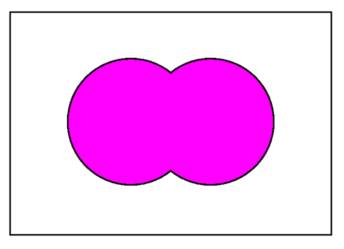
Now if event \(A\) is those outcomes having property \(X\) and \(B\) is those with property \(Y\text{,}\) the event \(A\cup B\text{,}\) with all outcomes in \(A\) together with all outcomes in \(B\) can be described as all outcomes satisfying \(X\) or \(Y\text{,}\) thus we sometimes pronounce the event “\(A\cup B\)” as “\(A\) or \(B\text{.}\)”
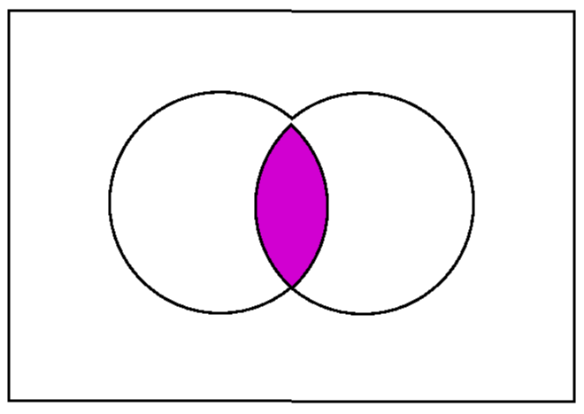
If, as before, event \(A\) consists of those outcomes having property \(X\) and \(B\) is those with property \(Y\text{,}\) the event \(A\cap B\) will consist of those outcomes which satisfy both \(X\) and \(Y\text{.}\) In other words, “\(A\cap B\)” can be described as “\(A\) and \(B\text{.}\)”
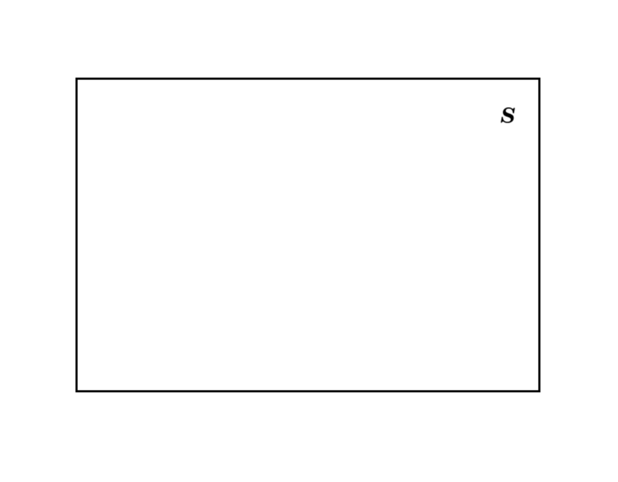
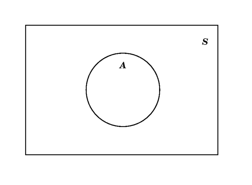
Venn diagrams are a simple way to display subsets of a fixed set and to show the relationships between these subsets and even the results of various set operations (like complement, union, and intersection) on them. The primary use we will make of Venn diagrams is for events in a certain sample space, so we will use that terminology [even though the technique has much wider application].
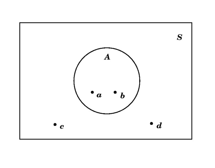
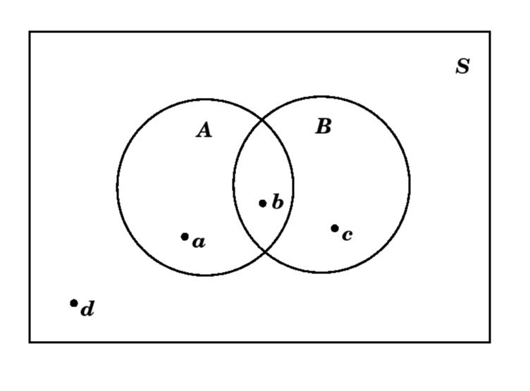
Sometimes, if the outcomes in the sample space \(S\) and in the event \(A\) might be indicated in the different parts of the Venn diagram. So, if \(S=\{a, b, c, d\}\) and \(A=\{a, b\}\subset S\text{,}\) we might draw this as
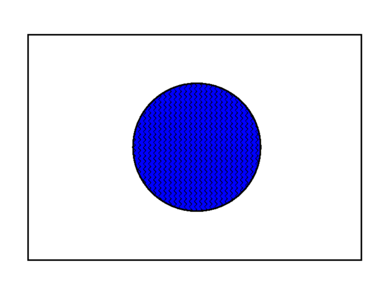
This can actually be helpful in figuring out what must be in \(E^c\text{.}\) In the example above with \(S=\{a, b, c, d\}\) and \(A=\{a, b\}\subset S\text{,}\) by looking at what is in the shaded exterior part for our picture of \(E^c\text{,}\) we can see that for that \(A\text{,}\) we would get \(A^c=\{c, d\}\text{.}\)
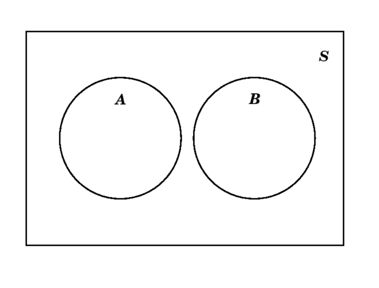
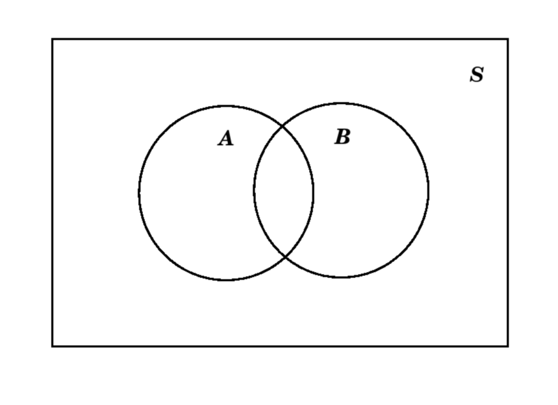
Moving now to set operations that work with two events, suppose we want to make a Venn diagram with events \(A\) and \(B\text{.}\) If we know these events are disjoint, then we would make the diagram as follows:
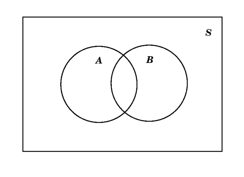
When in doubt, it is probably best to use the version with overlap, which then could simply not have any points in it (or could have zero probability, when we get to that, below).
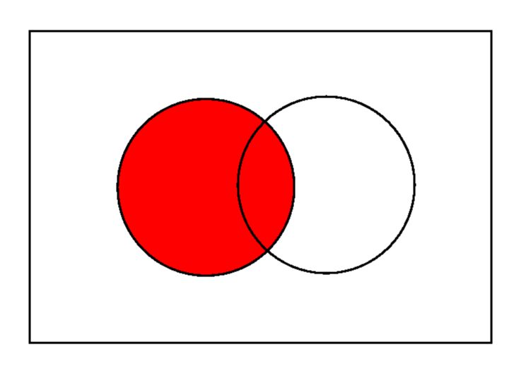
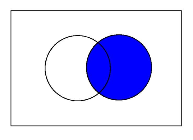
Figure4.23.Composite figure: Four diagrams illustrating union and intersection - filled circle A (top left), filled circle B (top right), both circles filled for A∪B (bottom left), and only overlap filled for A∩B (bottom right)
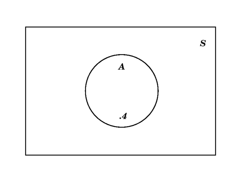
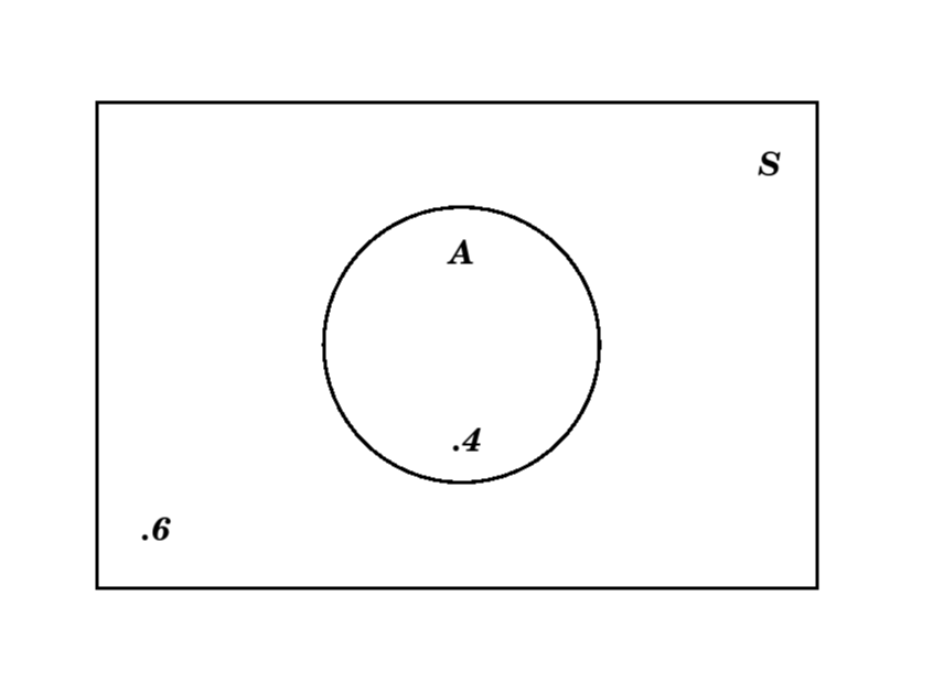
Another nice thing to do with Venn diagrams is to use them as a visual aid for probability computations. The basic idea is to make a diagram showing the various events sitting inside the usual rectangle, which stands for the sample space, and to put numbers in various parts of the diagram showing the probabilities of those events, or of the results of operations (unions, intersection, and complement) on those events.
But we can also put a number in the exterior of that circle which represents \(A\text{,}\) taking advantage of the fact that that exterior is \(A^c\) and the rule for probabilities of complements (point Item 3 in Definition 4.14) to conclude that the appropriate number is \(1-.4=.6\text{:}\)
We recommend that, in a Venn diagram showing probability values, you always put a number in the region exterior to all of the events [but inside the rectangle indicating the sample space, of course].
Complicating a little this process of putting probability numbers in the regions of a Venn diagram is the situation where we are giving for both an event and a subset of that event. This most often happens when we are told probabilities both of some events and of their intersection(s). Here is an example:
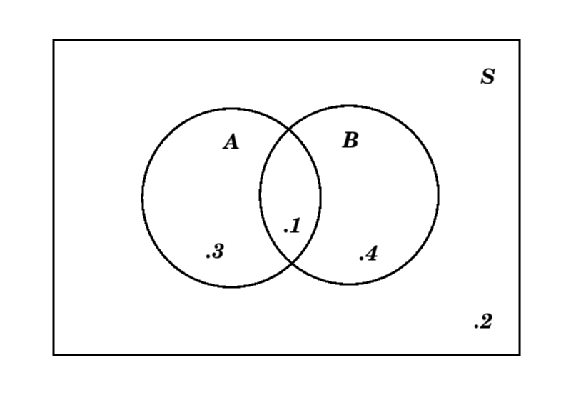
Suppose we are told that we have two events \(A\) and \(B\) in the sample space \(S\text{,}\) which satisfy \(P(A)=.4\text{,}\)\(P(B)=.5\text{,}\) and \(P(A\cap B)=.1\text{.}\) First of all, we know that \(A\) and \(B\) are not disjoint, since if they were disjoint, that would mean (by definition) that \(A\cap B=\emptyset\text{,}\) and since \(P(\emptyset)=0\) but \(P(A\cap B)\neq 0\text{,}\) that is not possible. So we draw a Venn diagram that we’ve see before:
However, it would be unwise simply to write those given numbers \(.4\text{,}\)\(.5\text{,}\) and \(.1\) into the three central regions of this diagram. The reason is that the number \(.1\) is the probability of \(A\cap B\text{,}\) which is a part of \(A\) already, so if we simply write \(.4\) in the rest of \(A\text{,}\) we would be counting that \(.1\) for the \(A\cap B\) twice. Therefore, before we write a number in the rest of \(A\text{,}\) outside of \(A\cap B\text{,}\) we have to subtract the \(.1\) for \(P(A\cap B)\text{.}\) That means that the number which goes in the rest of \(A\) should be \(.4-.1=.3\text{.}\) A similar reasoning tells us that the number in the part of \(B\) outside of \(A\cap B\text{,}\) should be \(.5-.1=.4\text{.}\) That means the Venn diagram with all probabilities written in would be:
The approach in the above example is our second important recommendation for who to put numbers in a Venn diagram showing probability values: always put a number in each region which corresponds to the probability of that smallest connected region containing the number, not any larger region.
One last point we should make, using the same argument as in the above example. Suppose we have events \(A\) and \(B\) in a sample space \(S\) (again). Suppose we are not sure if \(A\) and \(B\) are disjoint, so we cannot use the addition rule for disjoint events to compute \(P(A\cup B)\text{.}\) But notice that the events \(A\) and \(A^c\) are disjoint, so that \(A\cap B\) and \(A^c\cap B\) are also disjoint and
\begin{equation*}
A = A\cap S = A\cap\left(B\cup B^c\right) = \left(A\cap B\right)\cup\left(A\cap B^c\right)
\end{equation*}
is a decomposition of the event \(A\) into the two disjoint events \(A\cap B\) and \(A^c\cap B\text{.}\) From the addition rule for disjoint events, this means that
Here is a nice situation in which we can easily calculate a lot of probabilities fairly easily: if the sample space \(S\) of some experiment is finite.
So let’s suppose the sample space consists of just the outcomes \(S=\{o_1, o_2, \dots, o_n\}\text{.}\) For each of the outcomes, we can compute the probability:
Let’s think about what the rules for probability models tell us about these numbers \(p_1, p_2, \dots, p_n\text{.}\) First of all, since they are each the probability of an event, we see that
Furthermore, since \(S=\{o_1, o_2, \dots, o_n\}=\{o_1\}\cup\{o_2\}\cup \dots \cup\{o_n\}\) and all of the events \(\{o_1\}, \{o_2\}, \dots, \{o_n\}\) are disjoint, by the addition rule for disjoint events we have
The final thing to notice about this situation of a finite sample space is that if \(E\subset S\) is any event, then \(E\) will be just a collection of some of the outcomes from \(\{o_1, o_2, \dots, o_n\}\) (maybe none, maybe all, maybe an intermediate number). Since, again, the events like \(\{o_1\}\) and \(\{o_2\}\) and so on are disjoint, we can compute
\begin{align*}
P(E) &= P(\{\text{the outcomes } o_j \text{ which make up } E\})\\
&= \sum \{\text{the } p_j\text{'s for the outcomes in } E\}.
\end{align*}
A probability model on a sample space \(S\) with a finite number, \(n\text{,}\) of outcomes, is nothing other than a choice of real numbers \(p_1, p_2, \dots, p_n\text{,}\) all in the range from \(0\) to \(1\) and satisfying \(p_1+p_2+ \dots +p_n=1\text{.}\) For such a choice of numbers, we can compute the probability of any event \(E\subset S\) as
\begin{equation*}
P(E) = \sum \{\text{the } p_j\text{'s corresponding to the outcomes } o_j \text{ which make up } E\}.
\end{equation*}
For the coin flip of Example 4.2, there are only the two outcomes \(H\) and \(T\) for which we need to pick two probabilities, call them \(p\) and \(q\text{.}\) In fact, since the total must be \(1\text{,}\) we know that \(p+q=1\) or, in other words, \(q=1-p\text{.}\) The the probabilities for all events (which we listed in Example 4.9) are
What we’ve described here is, potentially, a biased coin, since we are not assuming that \(p=q\) — the probabilities of getting a head and a tail are not assumed to be the same. The alternative is to assume that we have a fair coin, meaning that \(p=q\text{.}\) Note that in such a case, since \(p+q=1\text{,}\) we have \(2p=1\) and so \(p=1/2\text{.}\) That is, the probability of a head (and, likewise, the probability of a tail) in a single throw of a fair coin is \(1/2\text{.}\)
As in the previous example, we can consider the die of Example 4.3 to a fair die, meaning that the individual face probabilities are all the same. Since they must also total to \(1\) (as we saw for all finite probability models), it follows that
When we are talking about dice, coins, individuals for some task, or another small, practical, finite experiment, we use the term fair to indicate that the probabilities of all individual outcomes are equal (and therefore all equal to the the number \(1/n\text{,}\) where \(n\) is the number of outcomes in the sample space). A more technical term for the same idea is equiprobable, while a more casual term which is often used for this in very informal settings is “at random” (such as “pick a card at random from this deck” or “pick a random patient from the study group to give the new treatment to…”).
Suppose we look at the experiment of Example 4.4 and add the information that the two dice we are rolling are fair. This actually isn’t quite enough to figure out the probabilities, since we also have to assure that the fair rolling of the first die doesn’t in any way affect the rolling of the second die. This is technically the requirement that the two rolls be independent, but since we won’t investigate that carefully until Section 4.2, below, let us instead here simply say that we assume the two rolls are fair and are in fact completely uninfluenced by anything around them in the world including each other.
What this means is that, in the long run, we would expect the first die to show a \(1\) roughly \({\frac16}^{\text{th}}\) of the time, and in the very long run, the second die would show a \(1\) roughly \({\frac16}^{\text{th}}\) of those times. This means that the outcome of the “roll two dice” experiment should be \(11\) with probability \(\frac{1}{36}\) — and the same reasoning would show that all of the outcomes have that probability. In other words, this is an equiprobable sample space with \(36\) outcomes each having probability \(\frac{1}{36}\text{.}\) Which in turn enables us to compute any probability we might like, such as
\begin{align*}
P(\text{"sum of the two rolls is 4"}) &= P(\{13, 22, 31\})\\
&= \frac{1}{36} + \frac{1}{36} + \frac{1}{36}\\
&= \frac{3}{36}\\
&= \frac{1}{12}.
\end{align*}
We have described the whole foundation of the theory of probability as coming from imperfect knowledge, in the sense that we don’t know for sure if an event \(A\) will happen any particular time we do the experiment but we do know, in the long run, in what fraction of times \(A\) will happen. Or, at least, we claim that there is some number \(P(A)\) such that after running the experiment \(N\) times, out of which \(n_A\) of these times are when \(A\) happened, \(P(A)\) is approximately \(n_A/N\) (and this ratio gets closer and closer to \(P(A)\) as \(N\) gets bigger and bigger).
But what if we have some knowledge? In particular, what happens if we know for sure that the event \(B\) has happened — will that influence our knowledge of whether \(A\) happens or not? As before, when there is randomness involved, we cannot tell for sure if \(A\) will happen, but we hope that, given the knowledge that \(B\) happened, we can make a more accurate guess about the probability of \(A\text{.}\)
If you pick a person at random in a certain country on a particular date, you might be able to estimate the probability that the person had a certain height if you knew enough about the range of heights of the whole population of that country. [In fact, below we will make estimates of this kind.] That is, if we define the event
\begin{equation*}
A=\text{"the random person is taller than 1.829 meters (6 feet)"}
\end{equation*}
\begin{equation*}
B=\text{"the random person's parents were both taller than 1.829 meters"}.
\end{equation*}
Because there is a genetic component to height, if you know that \(B\) happened, it would change your idea of how likely, given that knowledge, that \(A\) happened. Because genetics are not the only thing which determines a person’s height, you would not be certain that \(A\) happened, even given the knowledge of \(B\text{.}\)
Let us use the frequentist approach to derive a formula for this kind of probability of \(A\) given that \(B\) is known to have happened. So think about doing the repeatable experiment many times, say \(N\) times. Out of all those times, some times \(B\) happens, say it happens \(n_B\) times. Out of those times, the ones where \(B\) happened, sometimes \(A\) also happened. These are the cases where both \(A\) and \(B\) happened — or, converting this to a more mathematical descriptions, the times that \(A\cap B\) happened — so we will write it \(n_{A\cap B}\text{.}\)
We know that the probability of \(A\) happening in the cases where we know for sure that \(B\) happened is approximately \(n_{A\cap B}/n_B\text{.}\) Let’s do that favorite trick of multiplying and dividing by the same number, so finding that the probability in which we are interested is approximately
Building off of Example 4.30, note that the probability of rolling a \(2\) is \(P(\{2\})=1/6\) (as is the probability of rolling any other face — it’s a fair die). But suppose that you were told that the roll was even, which is the event \(\{2, 4, 6\}\text{,}\) and asked for the probability that the roll was a \(2\) given this prior knowledge. The answer would be
In other words, the probability of rolling a \(2\) on a fair die with no other information is \(1/6\text{,}\) which the probability of rolling a \(2\) given that we rolled an even number is \(1/3\text{.}\) So the probability doubled with the given information.
Sometimes the probability changes even more than merely doubling: the probability that we rolled a \(1\) with no other knowledge is \(1/6\text{,}\) while the probability that we rolled a \(1\) given that we rolled an even number is
But, actually, sometimes the conditional probability for some event is the same as the unconditioned probability. In other words, sometimes knowing that \(B\) happened doesn’t change our estimate of the probability of \(A\) at all, they are no really related events, at least from the point of view of probability. This motivates the
We can now fully explain what was going on in Example 4.32. The two fair dice were supposed to be rolled in a way that the first roll had no effect on the second — this exactly means that the dice were rolled independently. As we saw, this then means that each individual outcome of sample space \(S\) had probability \(\frac{1}{36}\text{.}\) But the first roll having any particular value is independent of the second roll having another, e.g., if \(A=\{11, 12, 13, 14, 15, 16\}\) is the event in that sample space of getting a \(1\) on the first roll and \(B=\{14, 24, 34, 44, 54, 64\}\) is the event of getting a \(4\) on the second roll, then events \(A\) and \(B\) are independent, as we check by using Fact:
On the other hand, the event “the sum of the rolls is \(4\text{,}\)” which is \(C=\{13, 22, 31\}\) as a set, is not independent of the value of the first roll, since \(P(A\cap C)=P(\{13\})=\frac{1}{36}\) but \(P(A)\cdot P(C)=\frac{6}{36}\cdot\frac{3}{36}=\frac16\cdot\frac{1}{12}=\frac{1}{72}\text{.}\)
Suppose we are doing a random experiment and there is some consequence of the result in which we are interested that can be measured by a number. The experiment might be playing a game of chance and the result could be how much you win or lose depending upon the outcome, or the experiment could be which part of the drivers’ manual you randomly choose to study and the result how many points we get on the driver’s license test we make the next day, or the experiment might be giving a new drug to a random patient in medical study and the result would be some medical measurement you make after treatment (blood pressure, white blood cell count, whatever), etc. There is a name for this situation in mathematics
A choice of a number for each outcome of a random experiment is called a random variable [RV]. If the values an RV takes can be counted, because they are either finite or countably infinite 1
A set is countably infinite if its elements can be put into a one-to-one correspondence with the natural numbers \(1, 2, 3, \ldots\text{.}\) For example, the set of all even positive integers \(\{2, 4, 6, \ldots\}\) is countably infinite.
in number, the RV is called discrete; if, instead, the RV takes on all the values in an interval of real numbers, the RV is called continuous.
We usually use capital letters to denote RVs and the corresponding lowercase letter to indicate a particular numerical value the RV might have, like \(X\) and \(x\text{.}\)
Suppose we play a silly game where you pay me $5 to play, then I flip a fair coin and I give you $10 if the coin comes up heads and $0 if it comes up tails. Then your net winnings, which would be +$5 or -$5 each time you play, are a random variable. Having only two possible values, this RV is certainly discrete.
Weather phenomena vary so much, due to such small effects — such as the famous butterfly flapping its wings in the Amazon rain forest causing a hurricane in North America — that they appear to be a random phenomenon. Therefore, observing the temperature at some weather station is a continuous random variable whose value can be any real number in some range like \(-100\) to \(100\) (we’re doing science, so we use \({}^\circ C\)).
Suppose we look at the “roll two fair dice independently” experiment from Example Example 4.38 and Example Example 4.32, which was based on the probability model in Example Example 4.32 and sample space in Example Example 4.4. Let us consider in this situation the random variable \(X\) whose value for some pair of dice rolls is the sum of the two numbers showing on the dice. So, for example, \(X(11)=2\text{,}\)\(X(12)=3\text{,}\)etc.
Given a discrete RV \(X\text{,}\) its distribution is a list of all of the values \(X\) takes on, together with the probability of it taking that value.
Let’s look at the RV, which we will call \(X\text{,}\) in the silly betting game of Example Example 4.40. As we noticed when we first defined that game, there are two possible values for this RV, $5 and -$5. We can actually think of “\(X=5\)” as describing an event, consisting of the set of all outcomes of the coin-flipping experiment which give you a net gain of $5. Likewise, “\(X=-5\)” describes the event consisting of the set of all outcomes which give you a net gain of -$5. These events are as follows:
What about the \(X=\text{``sum of the face values''}\) RV on the “roll two fair dice, independently” random experiment from Example Example 4.42? We have actually already done most of the work, finding out what values the RV can take and which outcomes cause each of those values. To summarize what we found:
But we have seen that this is an equiprobable situation, where the probability of any event \(A\) contain \(n\) outcomes is \(P(A)=n\cdot1/36\text{,}\) so we can instantly fill in the distribution table for this RV as
One thing to notice about distributions is that if we make a preliminary table, as we just did, of the events consisting of all outcomes which give a particular value when plugged into the RV, then we will have a collection of disjoint events which exhausts all of the sample space. What this means is that the sum of the probability values in the distribution table of an RV is the probability of the whole sample space of that RV’s experiment. Therefore
It is quite a good idea, whenever you write down a distribution, to check that this Fact is true in your distribution table, simply as a sanity check against simple arithmetic errors.
Since we cannot predict what exactly will be the outcome each time we perform a random experiment, we cannot predict with precision what will be the value of an RV on that experiment, each time. But, as we did with the basic idea of probability, maybe we can at least learn something from the long-term trends. It turns out that it is relatively easy to figure out the mean value of an RV over a large number of runs of the experiment.
Say \(X\) is a discrete RV, for which the distribution tells us that \(X\) takes the values \(x_1, \dots, x_n\text{,}\) each with corresponding probability \(p_1, \dots, p_n\text{.}\) Then the frequentist view of probability says that the probability \(p_i\) that \(X=x_i\) is (approximately) \(n_i/N\text{,}\) where \(n_i\) is the number of times \(X=x_i\) out of a large number \(N\) of runs of the experiment. But if
That means that, out of the \(N\) runs of the experiment, \(X\) will have the value \(x_1\) in \(p_1\,N\) runs, the value \(x_2\) in \(p_2\,N\) runs, etc. So the sum of \(X\) over those \(N\) runs will be
Therefore the mean value of \(X\) over these \(N\) runs will be the total divided by \(N\text{,}\) which is \(p_1\,x_1 + \dots + p_n x_n\text{.}\) This motivates the definition
Given a discrete RV \(X\) which takes on the values \(x_1, \dots, x_n\) with probabilities \(p_1, \dots, p_n\text{,}\) the expectation [sometimes also called the expected value] of \(X\) is the value
Note: The attentive reader will have noticed that we dealt above only with the case of a finite RV, not the case of a countably infinite one. It turns out that all of the above works quite well in that more complex case as well, so long as one is comfortable with a bit of mathematical technology called “summing an infinite series.” We do not assume such a comfort level in our readers at this time, so we shall pass over the details of expectations of infinite, discrete RVs.
Let’s compute the expectation of net profit RV \(X\) in the silly betting game of Example Example 4.40, whose distribution we computed in Example Example 4.44. Plugging straight into the definition, we see
In other words, your average net gain playing this silly game many times will be zero. Note that does not mean anything like “if you lose enough times in a row, the chances of starting to win again will go up,” as many gamblers seem to believe, it just means that, in the very long run, we can expect the average winnings to be approximately zero — but no one knows how long that run has to be before the balancing of wins and losses happens. 2
This is related to the Law of Large Numbers, which states that as the number of trials increases, the average of the results will converge to the expected value. However, there is no predetermined point at which this convergence must occur, and short-term deviations from the expected value are entirely normal.
In Example Example 4.47 we computed the distribution of the random variable \(X=\text{``sum of the face values''}\) on the “roll two fair dice, independently” random experiment from Example Example 4.42. It is therefore easy to plug the values of the probabilities and RV values from the distribution table into the formula for expectation, to get
So if you roll two fair dice independently and add the numbers which come up, then do this process many times and take the average, in the long run that average will be the value \(7\text{.}\)
Subsection4.3.4Density Functions for Continuous RVs
What about continuous random variables? Definition 4.43 of distribution explicitly excluded the case of continuous RVs, so does that mean we cannot do probability calculations in that case?
There is, when we think about it, something of a problem here. A distribution is supposed to be a list of possible values of the RV and the probability of each such value. But if some continuous RV has values which are an interval of real numbers, there is just no way to list all such numbers — it has been known since the late 1800s that there is no way to make a list like that[8]. In addition, the chance of some random process producing a real number that is exactly equal to some particular value really is zero: for two real numbers to be precisely equal requires infinite accuracy … think of all of those decimal digits, marching off in orderly rows to infinity, which must match between the two numbers.
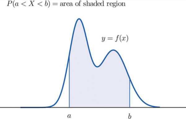
Let \(X\) be a continuous random variable whose values are the real interval \([x_{min},x_{max}]\text{,}\) where either \(x_{min}\) or \(x_{max}\) or both may be \(\infty\text{.}\) A [probability] density function for \(X\) is a function \(f(x)\) defined for \(x\) in \([x_{min},x_{max}]\text{,}\) meaning it is a curve with one \(y\) value for each \(x\) in that interval, with the property that
\begin{equation*}
P(a<X<b) = \left\{\begin{matrix}\text{the area in the } xy\text{-plane above the } x\text{-axis,}\\
\text{below the curve } y=f(x) \text{ and between } x=a \text{ and } x=b.\end{matrix}\right.\ .
\end{equation*}
If we want the idea of picking a real number on the interval \([x_{min},x_{max}]\) at random, where at random means that all numbers have the same chance of being picked (along the lines of fair in Definition 4.31, the height of the density function must be the same at all \(x\text{.}\) In other words, the density function \(f(x)\) must be a constant \(c\text{.}\) In fact, because of the above Fact, that constant must have the value \(\frac1{x_{max}-x_{min}}\text{.}\) There is a name for this:
The uniform distribution on \([x_{min},x_{max}]\) is the distribution for the continuous RV whose values are the interval \([x_{min},x_{max}]\) and whose density function is the constant function \(f(x)=\frac1{x_{max}-x_{min}}\text{.}\)
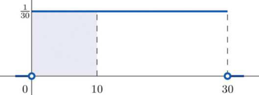
Suppose you take a bus to school every day and because of a chaotic home life (and, let’s face it, you don’t like mornings), you get to the bus stop at a pretty nearly perfectly random time. The bus also doesn’t stick perfectly to its schedule — but it is guaranteed to come at least every \(30\) minutes. What this adds up to is the idea that your waiting time at the bus stop is a uniformly distributed RV on the interval \([0,30]\text{.}\)
If you wonder one morning how likely it then is that you will wait for less than \(10\) minutes, you can simply compute the area of the rectangle whose base is the interval \([0,10]\) on the \(x\)-axis and whose height is \(\frac1{30}\text{,}\) which will be
One technical thing that can be confusing about continuous RVs and their density functions is the question of whether we should write \(P(a<X<b)\) or \(P(a\le X\le b)\text{.}\) But if you think about it, we really have three possible events here:
\begin{align*}
A &= \{\text{outcomes such that } X=a\},\\
M &= \{\text{outcomes such that } a<X<b\},\text{ and}\\
B &= \{\text{outcomes such that } X=b\}\ .
\end{align*}
Since \(X\) always takes on exactly one value for any particular outcome, there is no overlap between these events: they are all disjoint. That means that
\begin{equation*}
P(A\cup M\cup B) = P(A)+P(M)+P(B) = P(M)
\end{equation*}
where the last equality is because, as we said above, the probability of a continuous RV taking on exactly one particular value, as it would in events \(A\) and \(B\text{,}\) is \(0\text{.}\) The same would be true if we added merely one endpoint of the interval \((a,b)\text{.}\) To summarize:
As a consequence of this fact, some authors write probability formulæ about continuous RVs with “\(<\)” and some with “\(\le\)” and it makes no difference.
Suppose you repeatedly throw darts at a dartboard. You’re not a machine, so the darts hit in different places every time and you think of this as a repeatable random experiment whose outcomes are the locations of the dart on the board. You’re interested in the probabilities of getting close to the center of the board, so you decide for each experimental outcome (location of a dart you threw) to measure its distance to the center — this will be your RV \(X\text{.}\)
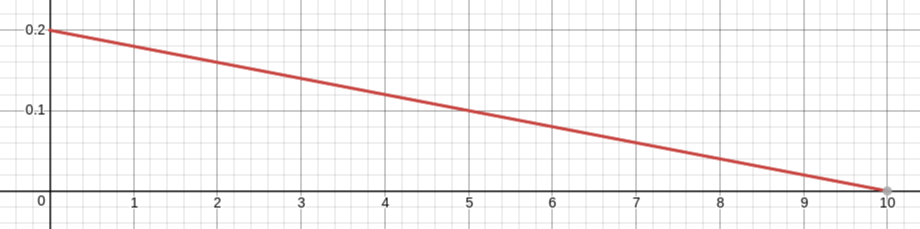
Being good at this game, you hit near the center more than near the edge and you never completely miss the board, whose radius is \(10cm\) — so \(X\) is more likely to be near \(0\) than near \(10\text{,}\) and it is never greater than \(10\text{.}\) What this means is that the RV has values forming the interval \([0,10]\) and the density function, defined on the same interval, should have its maximum value at \(x=0\) and should go down to the value \(0\) when \(x=10\text{.}\)
You decide to model this situation with the simplest density function you can think of that has the properties we just noticed: a straight line from the highest point of the density function when \(x=0\) down to the point \((10,0)\text{.}\) The figure that will result will be a triangle, and since the total area must be \(1\) and the base is \(10\) units long, the height must be \(.2\) units. [To get that, we solved the equation \(1=\frac12bh=\frac1210h=5h\) for \(h\text{.}\)] So the graph must be
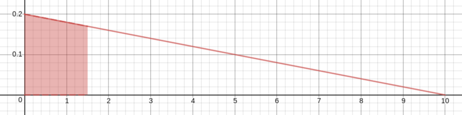
To the extent that you trust this model, you can now calculate the probabilities of events like, for example, “hitting the board within that center bull’s-eye of radius \(1.5cm\),” which probability would be the area of the shaded region in this graph:
The upper-right corner of this shaded region is at \(x\)-coordinate \(1.5\) and is on the line, so its \(y\)-coordinate is \(-\frac1{50}1.5+.2=.17\text{.}\) Since the region is a trapezoid, its area is the distance between the two parallel sides times the average of the lengths of the other two sides, giving
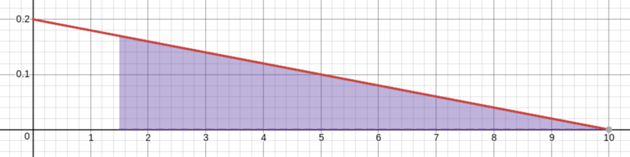
If you don’t remember the formula for the area of a trapezoid, you can do this problem another way: compute the probability of the complementary event, and then take one minus that number. The reason to do this would be that the complementary event corresponds to the shaded region here
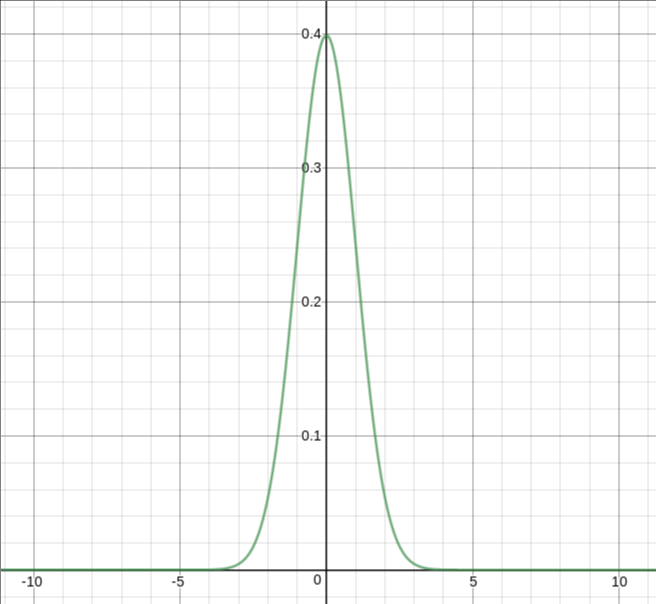
The Normal distribution with mean \(\mu_X\) and standard deviation \(\sigma_X\) is the continuous RV which takes on all real values and is governed by the probability density function
If \(X\) is a random variable which follows this distribution, then we say that \(X\) is Normally distributed with mean \(\mu_X\) and standard deviation \(\sigma_X\) or, in symbols, \(X\) is \(N(\mu_X, \sigma_X)\).
[More technical works also call this the Gaussian distribution, named after the great mathematician Carl Friedrich Gauss. But we will not use that term again in this book after this sentence ends.]
The good news about this complicated formula is that we don’t really have to do anything with it. We will collect some properties of the Normal distribution which have been derived from this formula, but these properties are useful enough, and other tools such as modern calculators and computers which can find specific areas we need under the graph of \(y=\rho(x)\text{,}\) that we won’t need to work directly with the above formula for \(\rho(x)\) again. It is nice to know that \(N(\mu_X, \sigma_X)\) does correspond to a specific, known density function, though, isn’t it?
The density function \(\rho\) for the Normal distribution \(N(\mu_X, \sigma_X)\) is a positive function for all values of \(x\) and the total area under the curve \(y=\rho(x)\) is \(1\text{.}\)
This means that \(N(\mu_X, \sigma_X)\) is a possible model for an RV \(X\) which tends to have one main, central value, and less often has other values farther away. That center is at the location given by the parameter \(\mu_X\text{,}\) so wherever we want to put the center of our model for \(X\text{,}\) we just use that for \(\mu_X\text{.}\)
This means that the amount \(X\) misses its center, \(\mu_X\text{,}\) tends to be about the same when it misses above \(\mu_X\) and when it misses below \(\mu_X\text{.}\) This would correspond to situations were you hit as much to the right as to the left of the center of a dartboard. Or when randomly picked people are as likely to be taller than the average height as they are to be shorter. Or when the time it takes a student to finish a standardized test is as likely to be less than the average as it is to be more than the average. Or in many, many other useful situations.
The density function \(\rho\) for the Normal distribution \(N(\mu_X, \sigma_X)\) has has tails in both directions which are quite thin, in fact get extremely thin as \(x\to\pm\infty\text{,}\) but never go all the way to \(0\text{.}\)
This means that \(N(\mu_X, \sigma_X)\) models situations where the amount \(X\) deviates from its average has no particular cut-off in the positive or negative direction. So you are throwing darts at a dart board, for example, and there is no way to know how far your dart may hit to the right or left of the center, maybe even way off the board and down the hall — although that may be very unlikely. Or perhaps the time it takes to complete some task is usually a certain amount, but every once and a while it might take much more time, so much more that there is really no natural limit you might know ahead of time.
At the same time, those tails of the Normal distribution are so thin, for values far away from \(\mu_X\text{,}\) that it can be a good model even for a situation where there is a natural limit to the values of \(X\) above or below \(\mu_X\text{.}\) For example, heights of adult males (in inches) in the United States are fairly well approximated by \(N(69, 2.8)\text{,}\) even though heights can never be less than \(0\) and \(N(69, 2.8)\) has an infinitely long tail to the left — because while that tail is non-zero all the way as \(x\to-\infty\text{,}\) it is very, very thin.
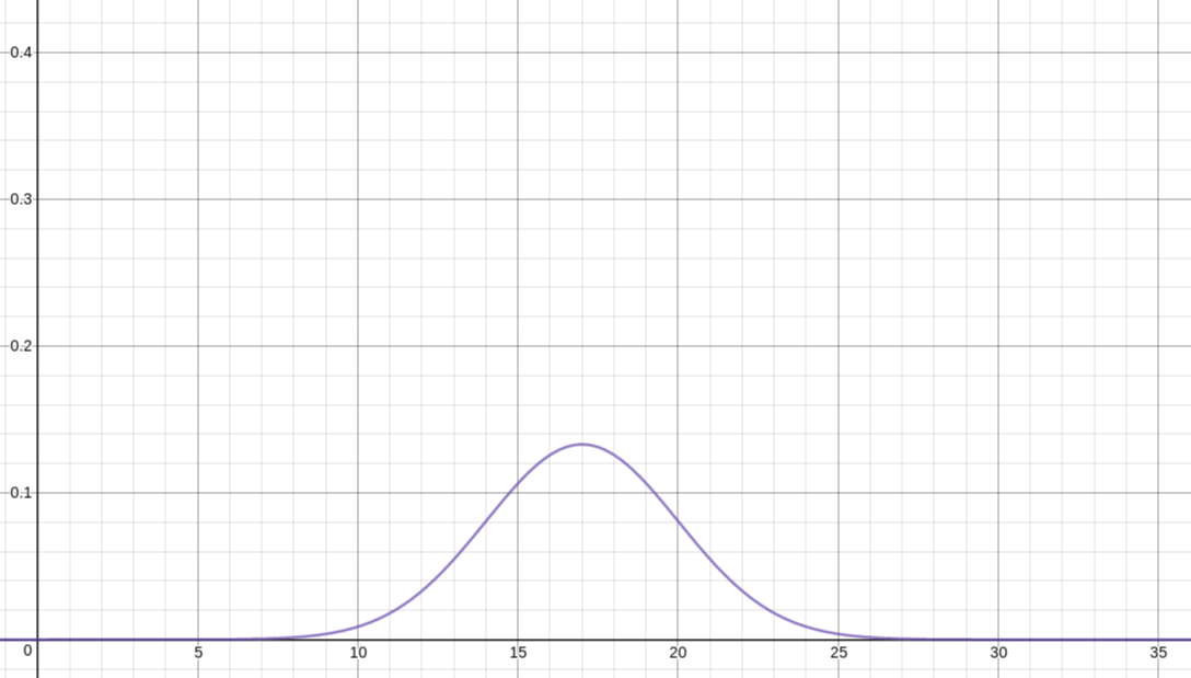
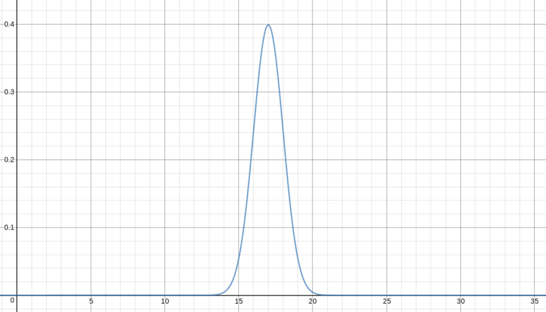
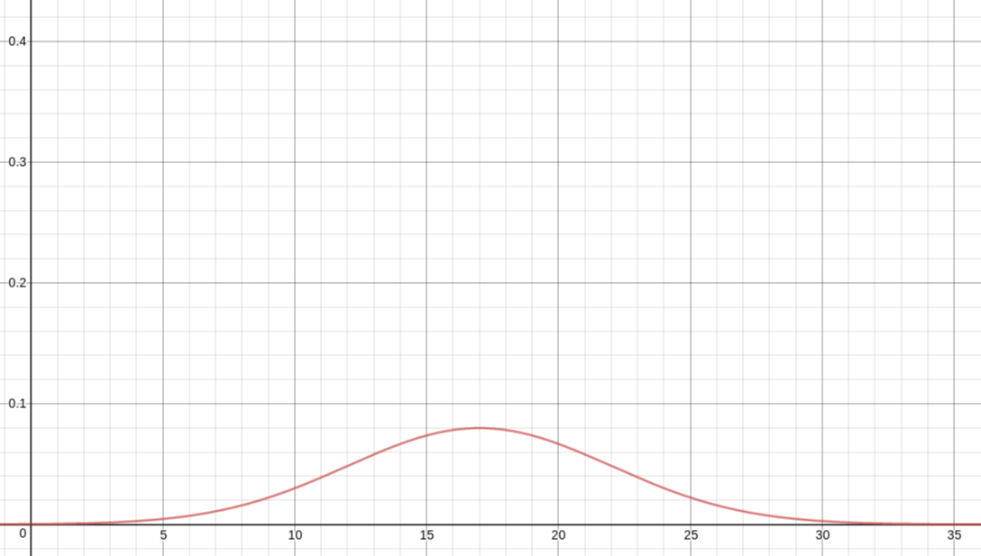
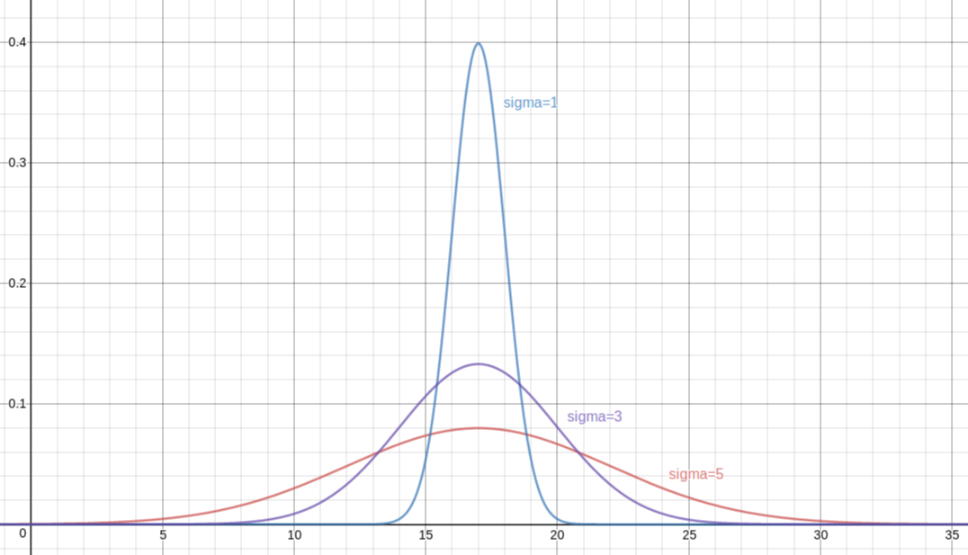
The graph of the density function \(\rho\) for the Normal distribution \(N(\mu_X, \sigma_X)\) has a taller and narrower peak if \(\sigma_X\) is smaller, and a lower and wider peak if \(\sigma_X\) is larger.
This allows the statistician to adjust how much variation there typically is in a normally distributed RV: By making \(\sigma_X\) small, we are saying that an RV \(X\) which is \(N(\mu_X, \sigma_X)\) is very likely to have values quite close to its center, \(\mu_X\text{.}\) If we make \(\sigma_X\) large, however, \(X\) is more likely to have values all over the place — still, centered at \(\mu_X\text{,}\) but more likely to wander farther away.
Let’s make a few versions of the graph we saw for \(\rho\) when \(\mu_X\) was \(17\) and \(\sigma_X\) was \(3\text{,}\) but now with different values of \(\sigma_X\text{.}\) First, if \(\sigma_X=1\text{,}\) we get
This variety of Normal distributions (one for each \(\mu_X\) and \(\sigma_X\)) is a bit bewildering, so traditionally, we concentrate on one particularly nice one.
The Normal distribution with mean \(\mu_X=0\) and standard deviation \(\sigma_X=1\) is called the standard Normal distribution and an RV [often written with the variable \(Z\)] that is \(N(0, 1)\) is described as a standard Normal RV.
The process of replacing a random variable \(X\) which is \(N(\mu_X, \sigma_X)\) with the standard normal RV \(Z=(X-\mu_X)/\sigma_X\) is called standardizing a Normal RV.
It used to be that standardization was an important step in solving problems with Normal RVs. A problem would be posed with information about some data that was modelled by a Normal RV with given mean \(\mu_X\) and standardization \(\sigma_X\text{.}\) Then questions about probabilities for that data could be answered by standardizing the RV and looking up values in a single table of areas under the standard Normal curve.
As we noted above, the heights of adult men in the United States, when measured in inches, give a RV \(X\) which is \(N(69, 2.8)\text{.}\) What percentage of the population, then, is taller than \(6\) feet?
First of all, the frequentist point of view on probability tells us that what we are interested in is the probability that a randomly chosen adult American male will be taller than \(6\) feet — that will be the same as the percentage of the population this tall. In other words, we must find the probability that \(X>72\text{,}\) since in inches, \(6\) feet becomes \(72\text{.}\) As \(X\) is a continuous RV, we must find the area under its density curve, which is the \(\rho\) for \(N(69, 2.8)\text{,}\) between \(72\) and \(\infty\text{.}\)
That \(\infty\) is a little intimidating, but since the tails of the Normal distribution are very thin, we can stop measuring area when \(x\) is some large number and we will have missed only a very tiny amount of area, so we will have a very good approximation. Let’s therefore find the area under \(\rho\) from \(x=72\) up to \(x=1000\text{.}\) This can be done in many ways:
which computes the area under the density function for \(N(\mu_X, \sigma_X)\) from \(-\infty\) to \(b\text{.}\) [The last input of “1” to NORM.DIST just tells it that we want to compute the area under the curve. If we used “0” instead, it would simple tell us the particular value of \(\rho(b)\text{,}\) which is of very direct little use in probability calculations.] Therefore, by doing \(1-NORM.DIST(72, 69, 2.8, 1)\text{,}\) we are taking the total area of 1 and subtracting the area to the left of 72, yielding the area to the right, as we wanted.
While standardizing a non-standard Normal RV and then looking up values in a table is an old-fashioned method that is tedious and no longer really needed, one old technique still comes in handy some times. It is based on the following:
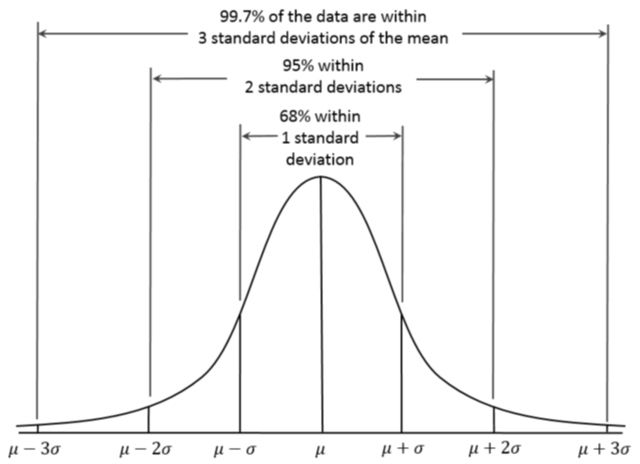
The 68-95-99.7 Rule: Let \(X\) be an \(N(\mu_X, \sigma_X)\) RV. Then some special values of the area under the graph of the density curve \(\rho\) for \(X\) are nice to know:
The area under the graph of \(\rho\) from \(x=\mu_X-\sigma_X\) to \(x=\mu_X+\sigma_X\text{,}\) also known as \(P(\mu_X-\sigma_X<X<\mu_X+\sigma_X)\text{,}\) is .68.
The area under the graph of \(\rho\) from \(x=\mu_X-2\sigma_X\) to \(x=\mu_X+2\sigma_X\text{,}\) also known as \(P(\mu_X-2\sigma_X<X<\mu_X+2\sigma_X)\text{,}\) is .95.
The area under the graph of \(\rho\) from \(x=\mu_X-3\sigma_X\) to \(x=\mu_X+3\sigma_X\text{,}\) also known as \(P(\mu_X-3\sigma_X<X<\mu_X+3\sigma_X)\text{,}\) is .997.
In order to use the 68-95-99.7 Rule in understanding a particular situation, it is helpful to keep an eye out for the numbers that it talks about. Therefore, when looking at a problem, one should notice if the numbers \(\mu_X+\sigma_X\text{,}\)\(\mu_X-\sigma_X\text{,}\)\(\mu_X+2\sigma_X\text{,}\)\(\mu_X-2\sigma_X\text{,}\)\(\mu_X+3\sigma_X\text{,}\) or \(\mu_X-3\sigma_X\) are ever mentioned. If so, perhaps this Rule can help.
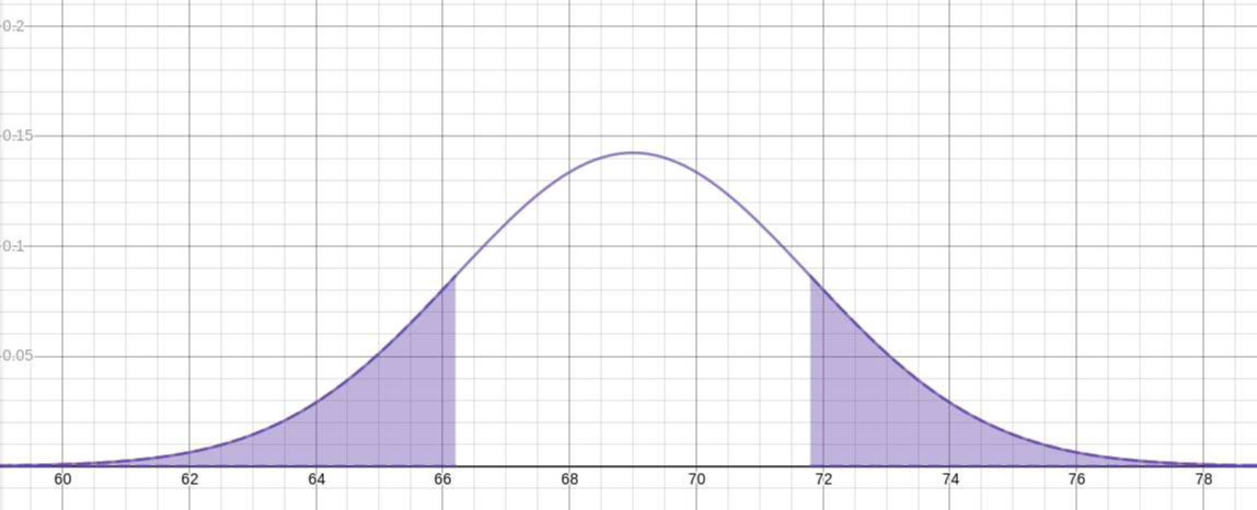
In Example Example 4.70, we needed to compute \(P(X>72)\) where \(X\) was known to be \(N(69, 2.8)\text{.}\) Is 72 one of the numbers for which we should be looking, to use the Rule? Well, it’s greater than \(\mu_X=69\text{,}\) so we could hope that it was \(\mu_X+\sigma_X\text{,}\)\(\mu_X+2\sigma_X\text{,}\) or \(\mu_X+3\sigma_X\text{.}\) But values are
Well, it is true that \(72\approx71.8\text{,}\) so we could use that fact and accept that we are only getting an approximate answer — an odd choice, given the availability of tools which will give us extremely precise answers, but let’s just go with it for a minute.
Since the event “\(X<66.2\)” is disjoint from the event “\(X>71.8\)” (\(X\) only takes on one value at a time, so it cannot be simultaneously less than 66.2 and greater than 71.8), we can use the simple rule for addition of probabilities:
Now, since the density function of the Normal distribution is symmetric around the line \(x=\mu_X\text{,}\) the two terms on the right in the above equation are equal, which means that
Let’s do one more computation in the context of the heights of adult American males, as in the immediately above Example Example 4.72, but now one in which the 68-95-99.7 Rule gives a more precise answer.
So say we are asked this time what proportion of adult American men are shorter than 63.4 inches. Why that height, in particular? Well, it’s how tall archaeologists have determined King Tut was in life. [No, that’s made up. It’s just a good number for this problem.]
Therefore, to answer what fraction of adult American males are shorter than 63.4 inches amounts to asking what is the value of \(P(X<\mu_X-2\sigma_X)\text{.}\)
What we know about \(\mu_X\pm2\sigma_X\) is that the probability of \(X\) being between those two values is \(P(\mu_X-2\sigma_X<X<\mu_X+2\sigma_X)=.95\text{.}\) As in the previous Example, the complementary event to “\(\mu_X-2\sigma_X<X<\mu_X+2\sigma_X\text{,}\)” which will have probability \(.05\text{,}\) consists of two pieces “\(X<\mu_X-2\sigma_X\)” and “\(X>\mu_X+2\sigma_X\text{,}\)” which have the same area by symmetry. Therefore
\begin{align*}
P(X<63.4)&=P(X<\mu_X-2\sigma_X)\\
&=\frac12\left[P(X<\mu_X-2\sigma_X)+P(X>\mu_X+2\sigma_X)\right]\\
&=\frac12P(X<\mu_X-2\sigma_X\text{ or }X>\mu_X+2\sigma_X)\text{ since they're disjoint}\\
&=\frac12P((\mu_X-2\sigma_X<X<\mu_X+2\sigma_X)^c)\\
&=\frac12\left[1-P(\mu_X-2\sigma_X<X<\mu_X+2\sigma_X)\right]\text{ by prob. for complements}\\
&=\frac12\,.05\\
&=.025
\end{align*}
Just the way finding the particular \(X\) values \(\mu_X\pm\sigma_X\text{,}\)\(\mu_X\pm2\sigma_X\text{,}\) and \(\mu_X\pm3\sigma_X\) in a particular situation would tell us the 68-95-99.7 Rule might be useful, so also would finding the probability values \(.68\text{,}\)\(.95\text{,}\)\(99.7\text{,}\) or their complements \(.32\text{,}\)\(.05\text{,}\) or \(.003\text{,}\) — or even half of one of those numbers, using the symmetry.
Notice that .15%, or the proportion .0015, is not one of the numbers in the 68-95-99.7 Rule, nor is it one of their complements — but it is half of one of the complements, being half of .003. Now, .003 is the complementary probability to .997, which was the probability in the range \(\mu_X\pm3\sigma_X\text{.}\) As we have seen already (twice), the complementary area to that in the region between \(\mu_X\pm3\sigma_X\) consists of two thin tails which are of equal area, each of these areas being \(\frac12(1-.997)=.0015\text{.}\) This all means that the beginning of that upper tail, above which value lies .15% of the population, is the \(X\) value \(\mu_X+3\sigma_X = 68 + 3\cdot2.8 = 77.4\text{.}\)
A basketball player shoots four free throws, and you write down the sequence of hits and misses. Write down the sample space for thinking of this whole thing as a random experiment.
In another game, a basketball player shoots four free throws, and you write down the number of baskets she makes. Write down the sample space for this different random experiment.
You take a normal, six-sided die, paint over all the sides, and then write the letter A on all six sides. You then roll the die. What is the sample space of this experiment? Also, list all the possible events for this experiment. [Hint: it may help to look at Example 4.9.]
One more time you paint over the sides, then write A on one third of the faces, B on one third of the other faces, and C on the remaining third. Again, give the sample space and all events.
The most common last [family] name in the world seems to be Wang [or the variant Wong]. Approximately 1.3% of the global population has this last name.
The most common first name in the world seems to be Mohammad [or one of several variants]. Some estimates suggest that perhaps as many as 2% of the global population has this first name.
Can you tell, from the above information, what percentage of the world population has the name “Mohammad Wang?” If so, why and what would it be? If not, why not, and can you make any guess about what that percentage would be, anyway?
[Hint: think of all the above percentages as probabilities, where the experiment is picking a random person on Earth and asking their name. Carefully describe some events for this experiment, relevant to this problem, and say what their probabilities are. Tell how combining events will or will not compute the probability of the desired event, corresponding to the desired percentage.]
[Note: don’t bet on the numbers given in this problem being too accurate — they might be, but there is a wide range of published values for them in public information from different sources, so probably they are only a very crude approximation.]
Suppose that when people have kids, the chance of having a boy or a girl is the same. Suppose also that the sexes of successive children in the same family are independent. [Neither of these is exactly true in real life, but let’s pretend for this problem.]
The Wang family has two children. If we think of the sexes of these children as the result of a random experiment, what is the sample space? Note that we’re interested in birth order as well, so that should be apparent from the sample space.
Suppose instead that we know that the Wangs’ older child is a boy. What is the probability, given this different information, that both Wang children are boys?
To solve this, clearly define events in words and with symbols, compute probabilities, and combine these to get the desired probability. Explain everything you do, of course.
Imagine you live on a street with a stop light at both ends of the block. You watch cars driving down the street and notice which ones have to stop at the \(1^{\text{st}}\) and/or \(2^{\text{nd}}\) light (or none). After counting cars and stops for a year, you have seen what a very large number — call it \(N\) — of cars did. Now imagine you decide to think about the experiment “pick a car on this street from the last year at random and notice at which light or lights it has to stop.”
Let \(A\) be the event “the car had to stop at the \(1^{\text{st}}\) light” and \(B\) be the event “the car had to stop at the \(2^{\text{nd}}\) light.” What else would you have to count, over your year of data collection, to estimate the probabilities of \(A\) and of \(B\text{?}\) Pick some numbers for all of these variables and show what the probabilities would then be.
Make a Venn diagram of this situation. Label each of the four connected regions of this diagram (the countries, if this were a map) with a number from \(\textcircled{1}\) to \(\textcircled{4}\text{,}\) then provide a key which gives, for each of these numbered regions, both a formula in terms of \(A\text{,}\)\(B\text{,}\) unions, intersections, and/or complements, and then also a description entirely in words which do not mention \(A\) or \(B\) or set operations at all. Then put a decimal number in each of the regions indicating the probability of the corresponding event.
Wait — for one of the regions, you can’t fill in the probability yet, with the information you’ve collected so far. What else would you have had to count over the data-collection year to estimate this probability? Make up a number and show what the corresponding probability would then be, and add that number to your Venn diagram.
Finally, using the probabilities you have chosen, are the events \(A\) and \(B\) independent? Why or why not? Explain in words what this means, in this context.
First of all, let’s make \(X\) represent the net gain a Lottery player would have for the various outcomes of playing — note that the ticket to play costs $2. How would you modify the above numbers to take into account the ticket costs?
Next, notice that the above table gives winning odds, not probabilities. How will you compute the probabilities from those odds? Recall that saying something has odds of “1 in \(n\)” means that it tends to happen about once out of \(n\) runs of the experiment. You might use the word frequentist somewhere in your answer here.
Finally, something is missing from the above table of outcomes. What prize — actually the most common one! — is missing from the table, and how will you figure out its probability?
After giving all of the above explanations, now write down the full, formal, probability distribution for this “net gain in EnergyCube Lottery plays” random variable, \(X\text{.}\)
In this problem, some of the numbers are quite small and will disappear entirely if you round them. So use a calculator or computer to compute everything here and keep as much accuracy as your device shows for each step of the calculation.
Continuing with the same scenario as in the previous Checkpoint 4.82, with the EnergyCube Lottery: What would be your expectation of the average gain per play of this Lottery? Explain fully, of course.
So if you were to play every weekday for a school year (so: five days a week for the 15 weeks of each semester, two semesters in the year), how much would you expect to win or lose in total?
Last problem in the situation of the above Checkpoint 4.82 about the EnergyCube Lottery: Suppose your friend plays the lottery and calls you to tell you that she won … but her cell phone runs out of charge in the middle of the call, and you don’t know how much she won. Given the information that she won, what is the probability that she won more than $1,000?
Let’s make a modified version of Example 4.58. You are again throwing darts at a dartboard, but you notice that you are very left-handed so your throws pull to the right much more than they pull to the left. What this means is that it is not a very good model of your dart throws just to notice how far they are from the center of the dartboard, it would be better to notice the \(x\)-coordinate of where the dart hits, measuring (in \(cm\)) with the center of the board at \(x\) location \(0\text{.}\) This will be your new choice of RV, which you will still call \(X\text{.}\)
You throw repeatedly at the board, measure \(X\text{,}\) and find out that you never hit more than \(10cm\) to the right of the center, while you are more accurate to the left and never hit more than \(5cm\) in that direction. You do hit the middle (\(X=0\)) the most often, and you guess that the probability decreases linearly to those edges where you never hit.
Now sketch the graph of the probability density function for \(X\text{.}\)[Hint: it will be a triangle, with one side along the interval of values \([x_{\min},x_{\max}]\) on the \(x\)-axis, and its maximum at the center of the dartboard.] Make sure that you put tick marks and numbers on the axes, enough so that the coordinates of the corners of the triangular graph can be seen easily. [Another hint: it is a useful fact that the total area under the graph of any probability density function is \(1\text{.}\)]
What is the probability that your next throw will be in the bull’s-eye, whose radius, remember, is \(1.5cm\) and which therefore stretches from \(x\) coordinate \(-1.5\) to \(x\)-coordinate \(1.5\text{?}\)
Here’s our last discussion of dartboards [maybe?]: One of the problems with the probability density function approaches from Example 4.58 and Checkpoint 4.86 is the assumption that the functions were linear (at least in pieces). It would be much more sensible to assume they were more bell-shaped, maybe like the Normal distribution.
Suppose your friend Mohammad Wang is an excellent dart-player. He throws at a board and you measure the \(x\)-coordinate of where the dart goes, as in Checkpoint 4.86 with the center corresponding to \(x=0\text{.}\) You notice that his darts are rarely — only 5% of the time in total! — more than \(5cm\) from the center of the board.
Fill in the blanks: “MW’s dart hits’ \(x\)-coordinates are an RV \(X\) which is Normally distributed with mean \(\mu_X=\)______ and standard deviation \(\sigma_X=\)______.” Explain, of course.
How often does he hit the bull’s-eye? Remember its radius is \(1.5cm\text{,}\) meaning that it stretches from \(x\) coordinate \(-1.5\) to \(x\)-coordinate \(1.5\text{.}\)