Skip to main content\(\newcommand{\R}{\mathbb{R}}
\newcommand{\lt}{<}
\newcommand{\gt}{>}
\newcommand{\amp}{&}
\definecolor{fillinmathshade}{gray}{0.9}
\newcommand{\fillinmath}[1]{\mathchoice{\colorbox{fillinmathshade}{$\displaystyle \phantom{\,#1\,}$}}{\colorbox{fillinmathshade}{$\textstyle \phantom{\,#1\,}$}}{\colorbox{fillinmathshade}{$\scriptstyle \phantom{\,#1\,}$}}{\colorbox{fillinmathshade}{$\scriptscriptstyle\phantom{\,#1\,}$}}}
\)
Section 13.4 Distributions
Subsection 13.4.1 Normal changing mean
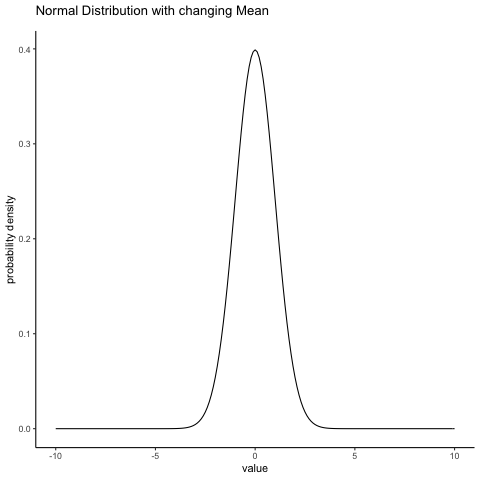
Figure 13.4.1. Normal distribution with changing mean
some_means<-c(0,1,2,3,4,5,4,3,2,1)
all_df<-data.frame()
for(i in 1:10){
  dnorm_vec <- dnorm(seq(-10,10,.1),mean=some_means[i],sd=1)
  x_range   <- seq(-10,10,.1)
  means <- rep(some_means[i], length(x_range))
  sims <- rep(i, length(x_range))
  t_df<-data.frame(sims,means,x_range,dnorm_vec)
  all_df<-rbind(all_df,t_df)
}

ggplot(all_df, aes(x=x_range,y=dnorm_vec))+
  geom_line()+
  theme_classic()+
  ylab("probability density")+
  xlab("value")+
  ggtitle("Normal Distribution with changing Mean")+
   transition_states(
    sims,
    transition_length = 1,
    state_length = 1
  )
Subsection 13.4.2 Normal changing sd
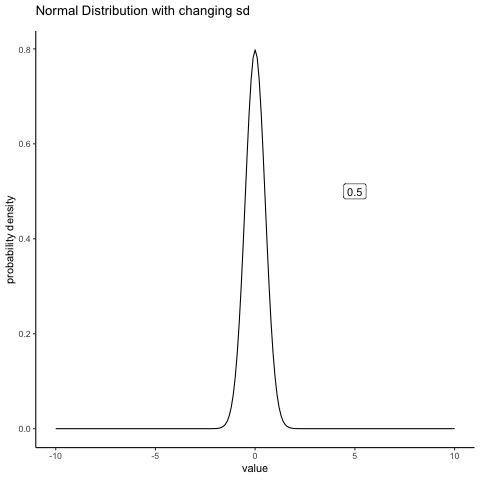
Figure 13.4.2. Normal distribution with changing standard deviation
some_sds<-seq(0.5,5,.5)
all_df<-data.frame()
for(i in 1:10){
  dnorm_vec <- dnorm(seq(-10,10,.1),mean=0,sd=some_sds[i])
  x_range   <- seq(-10,10,.1)
  sds <- rep(some_sds[i], length(x_range))
  sims <- rep(i, length(x_range))
  t_df<-data.frame(sims,sds,x_range,dnorm_vec)
  all_df<-rbind(all_df,t_df)
}

labs_df<-data.frame(sims=1:10,
                    sds=as.character(seq(0.5,5,.5)))

ggplot(all_df, aes(x=x_range,y=dnorm_vec, frame=sims))+
  geom_line()+
  theme_classic()+
  ylab("probability density")+
  xlab("value")+
  ggtitle("Normal Distribution with changing sd")+
  geom_label(data = labs_df, aes(x = 5, y = .5, label = sds))+
   transition_states(
    sims,
    transition_length = 2,
    state_length = 1
  )+
  enter_fade() +
  exit_shrink() +
  ease_aes('sine-in-out')