X <- c(
  seq(-5, 5, .1),
  seq(-5, 5, .1),
  seq(-5, 5, .1),
  seq(-5, 5, .1),
  seq(-5, 5, .1),
  seq(-5, 5, .1),
  seq(-5, 5, .1),
  seq(-5, 5, .1)
)
Y <- c(
  dnorm(seq(-5, 5, .1), 0, 1),
  dnorm(seq(-5, 5, .1), 0, 1),
  dnorm(seq(-5, 5, .1), 0, 1),
  dnorm(seq(-5, 5, .1), .5, 1),
  dnorm(seq(-5, 5, .1), 0, 1),
  dnorm(seq(-5, 5, .1), 1, 1),
  dnorm(seq(-5, 5, .1), 0, 1),
  dnorm(seq(-5, 5, .1), 2, 1)
)
effect_size <- rep(c(0, .5, 1, 2), each = 101 * 2)
condition <- rep(rep(c("A", "B"), each = 101), 2)
df <- data.frame(effect_size,
                 condition,
                 X, Y)

ggplot(df, aes(
  x = X,
  y = Y,
  group = condition,
  color = condition
)) +
  geom_line() +
  theme_classic(base_size = 15) +
  facet_wrap( ~ effect_size) +
  xlab("values") +
  ylab("density")
Section 12.1 Effect-size and power
So far we neglected to discuss the topic of effect-size, and we barely talked about statistical power. We will talk a little bit about these things here.
First, it is worth pointing out that over the years, at least in Psychology, many societies and journals have made recommendations about how researchers should report their statistical analyses. A common recommendation is that measures of “effect size” should be reported. Similarly, many journals now require that researchers report an “a priori” power-analysis (the recommendation is that this should be done before the data is collected). Because these recommendations are so prevalent it is worth discussing what these ideas refer to. At the same time, the meaning of effect-size and power somewhat depend on your “philosophical” bent. For these complicating reasons we have suspended our discussion of the topic until now.
The practice of using measures of effect size and conducting power-analyses are also good examples of the more general need to think about your intentions for your analysis. If you are going to report effect size and conduct power analyses, we caution against doing so automatically simply because someone else recommends that you do them. Instead, these activities and other suitable ones should be done as a part of justifying what you are doing. It is a part of thinking about how to make your data answer questions for you.
Subsection 12.1.1 Chance vs. real effects
Let’s rehash something we’ve said over and over again. First, researchers are interested in whether their manipulation causes a change in their measurement. If they can be confident it does, then they have uncovered a causal force (the manipulation). However, we know that differences in the measurement between experimental conditions can arise by chance alone, just by sampling error. In fact, we can create pictures that show us the window of chance for a given statistic, these tells us roughly the range and likelihoods of getting various differences just by chance. With these windows in hand, we can then determine whether a difference between conditions was likely or unlikely to be due to chance. We also learned that sample-size plays a big role in the shape of the chance window. Small samples allow chance larger opportunities to make big differences. Large samples deprive chance of opportunities to make big differences. The general lesson up to this point has been to design an experiment with a large enough sample to detect the effect of interest. If your design isn’t well formed, you could easily be measuring noise, and your differences could be caused by sampling error. Generally speaking, this is still a very good lesson: better designs produce better data; and, you can’t fix a broken design with statistics.
One missing consideration from the above is the size of the effect itself. For example, consider a manipulation in terms of the size of its hammer. A strong manipulation is like a jack-hammer: it is loud, strong, and capable of producing big effects like breaking up concrete. A medium manipulation is like a regular hammer: it works, you can hear it, it can reliably drive a nail into wood. A small manipulation is like tapping something with a pencil: it does something, you can barely hear it, and only in a quiet room. Finally, a really small effect would be hammering something with a feather, it leaves almost no mark and does nothing to wood or concrete. The lesson is, if you want to break up concrete, use a jack-hammer; or, if you want to measure your effect, make your manipulation stronger (like a jack-hammer if you can) so it produces a bigger difference.
Subsection 12.1.2 Effect size: concrete vs. abstract notions
When considering the magnitude of an effect (i.e., the size of the effect) it is useful to keep the question “compared to what?” in the back of your mind. The “compared to what?” question prompts a critical evaluation of both the object of comparison and what the relative differences in size actually refer to.
Sometimes a measure of effect size can be fairly concrete and straightforward to interpret. For example, consider a magic manipulation that reliably improves test performance on most university exams by 5%. Although a 5% increase might be small in another context, in the context of exams it could be a whole letter grade, and students might be interested to learn more about the manipulation to improve their grades. Othertimes a measure of effect size might be more abstract and less straightforward to interpret. For example, a miracle drug might reduce the risk of some disease by 100%. This sounds like a big effect, but we should ask compared to what? If the disease is already extremely rare and without the drug only 2 people in 10 million contract the disease, and with the drug 1 person out of 10 million contracts the disease; then, yes, the drug does produce a 100% reduction (from 2 to 1 per 10 million), but the original chances of getting the disease were extremely unlikely in the first place. In other words, reframing the 100% decrease in terms of the base rates establishes the object comparison and shows the relative sizes more clearly.
Let’s talk about concrete measures some more. How about learning a musical instrument? Let’s say it takes 10,000 hours to become an expert piano, violin, or guitar player. And, let’s say you found a training program on the internet claiming that by subscribing to their method you will learn the instrument in less time than normal. That is a claim about the effect size of their method. You would want to know how big the effect is right? For example, the effect-size could be 10 hours. That would mean it would take you 9,980 hours to become an expert (that’s a whole 10 hours less). If I knew the effect-size was so tiny, I wouldn’t bother with their new method. But, if the effect size was say 1,000 hours, that’s a pretty big deal, that’s 10% less (still doesn’t seem like much, but saving 1,000 hours might be worth it).
Just as we have concrete measures that are readily interpretable, Psychology produces measures that are extremely difficult to interpret. For example, questionnaire measures often have no concrete meaning and only an abstract statistical meaning. If you wanted to know whether a manipulation caused people to become more or less happy and you used to questionnaire to measure happiness, you might find that people were “50” happy in condition 1, and “60” happy in condition 2, that’s a difference of 10 happy units. But how much is “10” happy units? Is that a big or small difference? It’s not immediately obvious. What is the solution here? One solution is to provide a standardized measure of the difference, like a z-score. For example, if a difference of 10 reflected a shift of one standard deviation that would be useful to know, and that would be a sizeable shift. If the difference was only a .1 shift in terms of standard deviation, then the difference of 10 wouldn’t be very large. We elaborate on this idea next in describing Cohen’s d.
Subsection 12.1.3 Cohen’s d
Let’s look a few distributions to firm up some ideas about effect-size. Figure 12.1.2 has four panels. The first panel (0) represents the null distribution of no differences. This is the idea that your manipulation A vs. B doesn’t do anything at all, as a result when you measure scores in conditions A and B, you are effectively sampling scores from the very same overall distribution. The panel shows the distribution as green for condition B, but the red one for condition A is identical and drawn underneath (it’s invisible). There is 0 difference between these distributions, so it represent a null effect.
Remark 12.1.1. R Code.
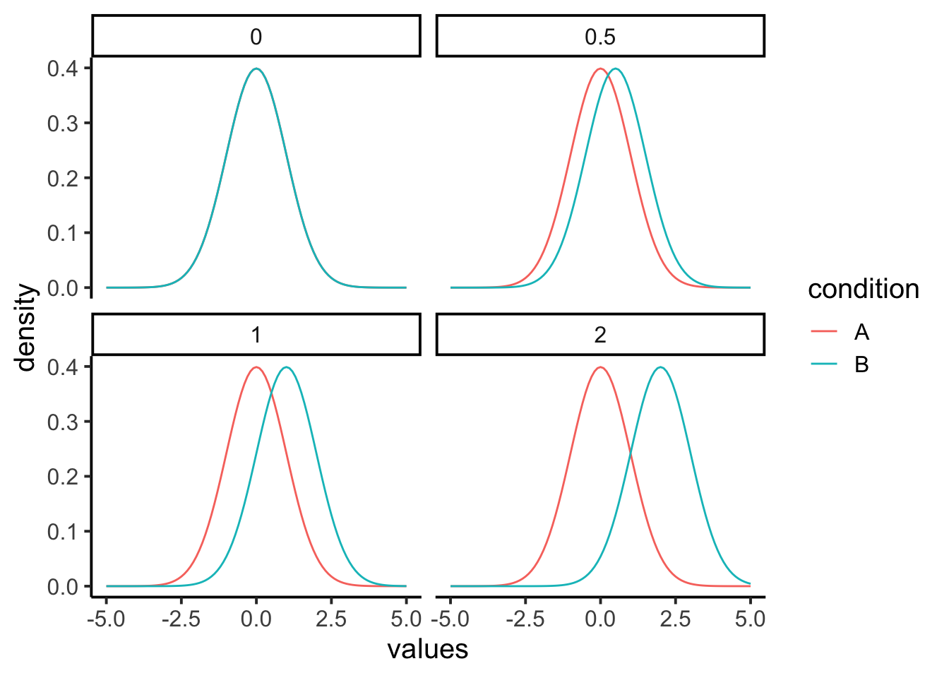
The remaining panels are hypothetical examples of what a true effect could look like, when your manipulation actually causes a difference. For example, if condition A is a control group, and condition B is a treatment group, we are looking at three cases where the treatment manipulation causes a positive shift in the mean of the distribution. We are using normal curves with mean = 0 and sd =1 for this demonstration, so a shift of .5 is a shift of half of a standard deviation. A shift of 1 is a shift of 1 standard deviation, and a shift of 2 is a shift of 2 standard deviations. We could draw many more examples showing even bigger shifts, or shifts that go in the other direction.
Let’s look at another example, but this time we’ll use some concrete measurements. Let’s say we are looking at final exam performance, so our numbers are grade percentages. Let’s also say that we know the mean on the test is 65%, with a standard deviation of 5%. Group A could be a control that just takes the test, Group B could receive some “educational” manipulation designed to improve the test score. These graphs then show us some hypotheses about what the manipulation may or may not be doing.
Remark 12.1.3. R Code.
X <- c(
  seq(25, 100, 1),
  seq(25, 100, 1),
  seq(25, 100, 1),
  seq(25, 100, 1),
  seq(25, 100, 1),
  seq(25, 100, 1),
  seq(25, 100, 1),
  seq(25, 100, 1)
)
Y <- c(
  dnorm(seq(25, 100, 1), 65, 5),
  dnorm(seq(25, 100, 1), 65, 5),
  dnorm(seq(25, 100, 1), 65, 5),
  dnorm(seq(25, 100, 1), 67.5, 5),
  dnorm(seq(25, 100, 1), 65, 5),
  dnorm(seq(25, 100, 1), 70, 5),
  dnorm(seq(25, 100, 1), 65, 5),
  dnorm(seq(25, 100, 1), 75, 5)
)
effect_size <-
  rep(c("65, d=0", "67.5,d=.5", "70, d=1", "75, d=2"), each = 76 * 2)
condition <- rep(rep(c("A", "B"), each = 76), 2)
df <- data.frame(effect_size,
                 condition,
                 X, Y)

ggplot(df, aes(
  x = X,
  y = Y,
  group = condition,
  color = condition
)) +
  geom_line() +
  theme_classic(base_size = 15) +
  facet_wrap( ~ effect_size) +
  xlab("values") +
  ylab("density")
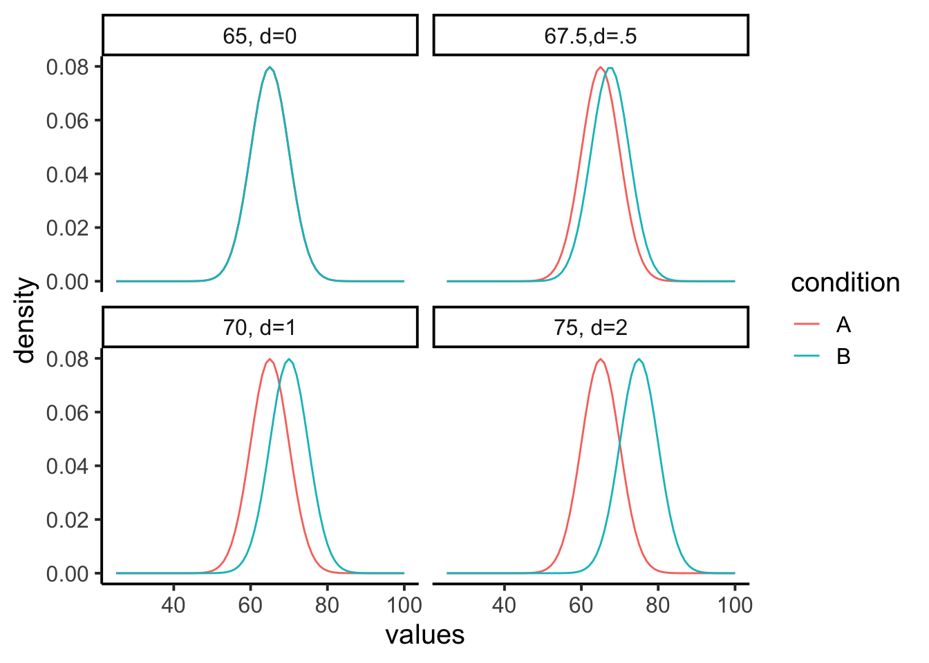
The first panel shows that both condition A and B will sample test scores from the same distribution (mean = 65, with 0 effect). The other panels show shifted mean for condition B (the treatment that is supposed to increase test performance). So, the treatment could increase the test performance by 2.5% (mean 67.5, .5 sd shift), or by 5% (mean 70, 1 sd shift), or by 10% (mean 75%, 2 sd shift), or by any other amount. In terms of our previous metaphor, a shift of 2 standard deviations is more like jack-hammer in terms of size, and a shift of .5 standard deviations is more like using a pencil. The thing about research, is we often have no clue about whether our manipulation will produce a big or small effect, that’s why we are conducting the research.
You might have noticed that the letter \(d\) appears in the above figure. Why is that? Jacob Cohen [(Cohen, 1988)] used the letter \(d\) in defining the effect-size for this situation, and now everyone calls it Cohen’s \(d\text{.}\) The formula for Cohen’s \(d\) is:
\(d = \frac{\text{mean for condition 1} - \text{mean for condition 2}}{\text{population standard deviation}}\)
If you notice, this is just a kind of z-score. It is a way to standardize the mean difference in terms of the population standard deviation.
It is also worth noting again that this measure of effect-size is entirely hypothetical for most purposes. In general, researchers do not know the population standard deviation, they can only guess at it, or estimate it from the sample. The same goes for means, in the formula these are hypothetical mean differences in two population distributions. In practice, researchers do not know these values, they guess at them from their samples.
Before discussing why the concept of effect-size can be useful, we note that Cohen’s \(d\) is useful for understanding abstract measures. For example, when you don’t know what a difference of 10 or 20 means as a raw score, you can standardize the difference by the sample standard deviation, then you know roughly how big the effect is in terms of standard units. If you thought a 20 was big, but it turned out to be only 1/10th of a standard deviation, then you would know the effect is actually quite small with respect to the overall variability in the data.
