The
duke_forest data can be found in the openintro R package.
duke_forest data can be found in the openintro R package.
duke_forest.| price | bed | bath | area | year_built | cooling | lot |
|---|---|---|---|---|---|---|
| 1,520,000 | 3 | 4 | 6,040 | 1972 | central | 0.46 |
| 1,030,000 | 5 | 4.5 | 4,475 | 1969 | central | 1.14 |
| 420,000 | 2 | 2.5 | 1,745 | 1959 | central | 0.51 |
| 680,000 | 4 | 3 | 2,091 | 1961 | other | 0.84 |
duke_forest dataset.| Variable | Description |
|---|---|
price |
Sale price, in USD |
bed |
Number of bedrooms |
bath |
Number of bathrooms |
area |
Area of home, in square feet |
year_built |
Year the home was built |
cooling |
Cooling system: central or other (other is baseline) |
lot |
Area of the entire property, in acres |
price
pr_bed <- ggplot(duke_forest, aes(x = bed, y = price)) +
  geom_point(alpha = 0.8) +
  labs(
    x = "Number of bedrooms",
    y = "Sale price (USD)"
  ) +
  stat_cor(aes(label = paste("r", ..r.., sep = "~`=`~"))) +
  scale_y_continuous(labels = label_dollar(scale = 1/1000, suffix = "K"))

pr_bath <- ggplot(duke_forest, aes(x = bath, y = price)) +
  geom_point(alpha = 0.8) +
  labs(
    x = "Number of bathrooms",
    y = "Sale price (USD)"
  ) +
  stat_cor(aes(label = paste("r", ..r.., sep = "~`=`~"))) +
  scale_y_continuous(labels = label_dollar(scale = 1/1000, suffix = "K"))

pr_area <- ggplot(duke_forest, aes(x = area, y = price)) +
  geom_point(alpha = 0.8) +
  labs(
    x = "Area of home (in square feet)",
    y = "Sale price (USD)"
  ) +
  stat_cor(aes(label = paste("r", ..r.., sep = "~`=`~"))) +
  scale_y_continuous(labels = label_dollar(scale = 1/1000, suffix = "K"))

pr_year <- ggplot(duke_forest, aes(x = year_built, y = price)) +
  geom_point(alpha = 0.8) +
  labs(
    x = "Year built",
    y = "Sale price (USD)"
  ) +
  stat_cor(aes(label = paste("r", ..r.., sep = "~`=`~"))) +
  scale_y_continuous(labels = label_dollar(scale = 1/1000, suffix = "K"))

pr_cool <- ggplot(duke_forest, aes(x = cooling, y = price)) +
  geom_point(alpha = 0.8) +
  labs(
    x = "Cooling type",
    y = "Sale price (USD)"
  ) +
  stat_cor(aes(label = paste("r", ..r.., sep = "~`=`~"))) +
  scale_y_continuous(labels = label_dollar(scale = 1/1000, suffix = "K"))

pr_lot <- ggplot(duke_forest, aes(x = lot, y = price)) +
  geom_point(alpha = 0.8) +
  labs(
    x = "Area of property (in acres)",
    y = "Sale price (USD)"
  ) +
  stat_cor(aes(label = paste("r", ..r.., sep = "~`=`~"))) +
  scale_y_continuous(labels = label_dollar(scale = 1/1000, suffix = "K"))

pr_bed + pr_bath + pr_area + pr_year + pr_cool + pr_lot +
  plot_layout(ncol = 2)
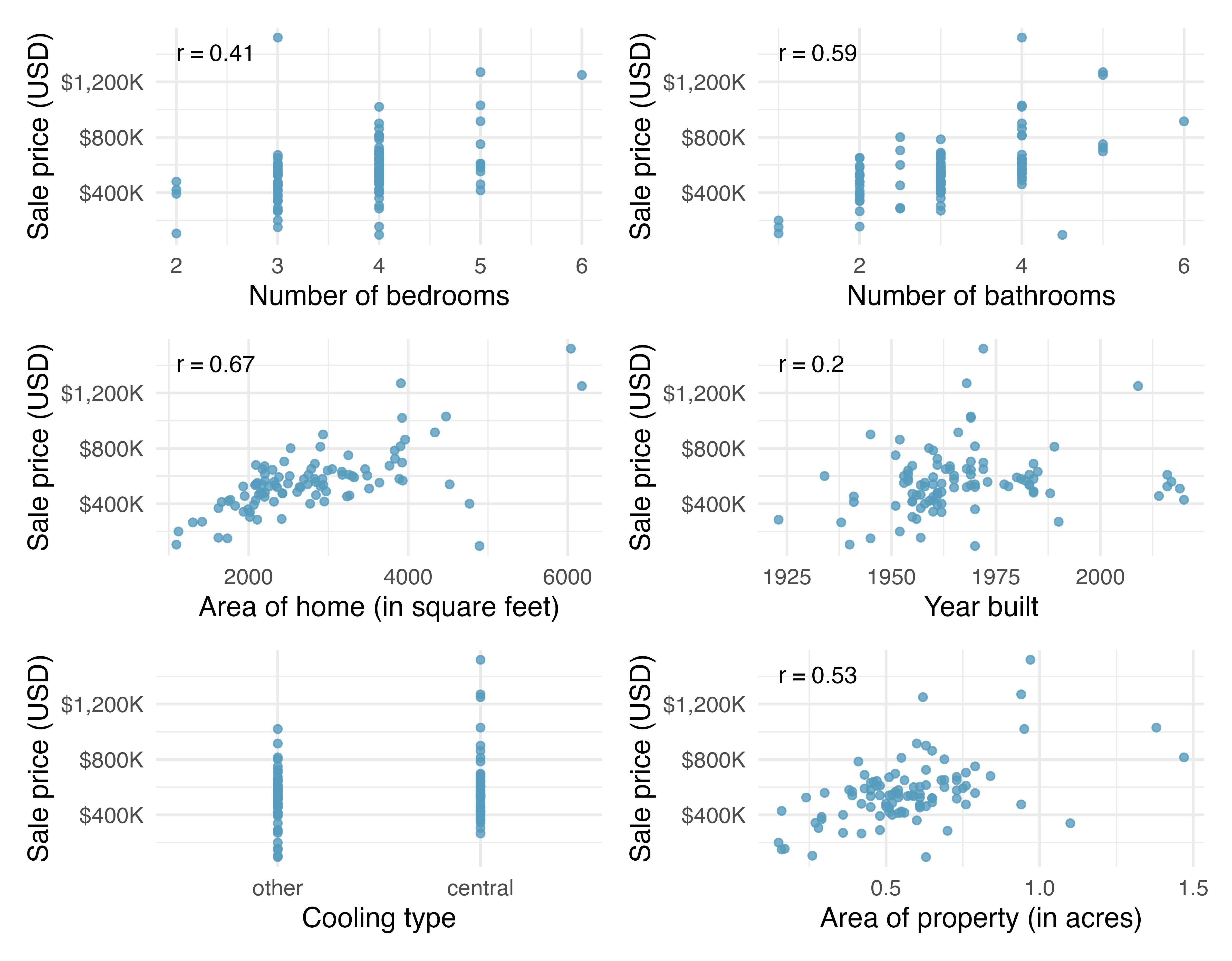
cooling. Why not? Can the variable still be used in the linear model?
cooling is categorical, not numerical. It can, however, be used in the linear model as a binary indicator variable coded, for example, with a \(1\) for central and \(0\) for other.
area of the home is the variable which is most highly correlated with price. Additionally, the scatterplot for price vs. area seems to show a strong linear relationship between the two variables. Note that the correlation coefficient and the scatterplot linearity will often give the same conclusion. However, recall that the correlation coefficient is very sensitive to outliers, so it is always wise to look at the scatterplot even when the variables are highly correlated.
price with area
price from area. The resulting model information is given in Table 10.8.
| term | estimate | std.error | statistic | p.value |
|---|---|---|---|---|
(Intercept) |
116,652 | 53,302 | 2.19 | 0.0316 |
area |
159 | 18 | 8.78 | <0.0001 |
| Adjusted R-sq = 0.4399 | ||||
| df = 96 | ||||
duke_forest |>
  lm(price ~ area, data = _) |>
  augment() |>
  ggplot(aes(x = .fitted, y = .resid)) +
  geom_point(size = 2, alpha = 0.8) +
  labs(
    x = "Predicted values of sale price (in USD)",
    y = "Residuals"
  ) +
  geom_hline(yintercept = 0, linetype = "dashed") +
  scale_x_continuous(labels = label_dollar(scale = 1/1000, suffix = "K")) +
  scale_y_continuous(labels = label_dollar(scale = 1/1000, suffix = "K"))
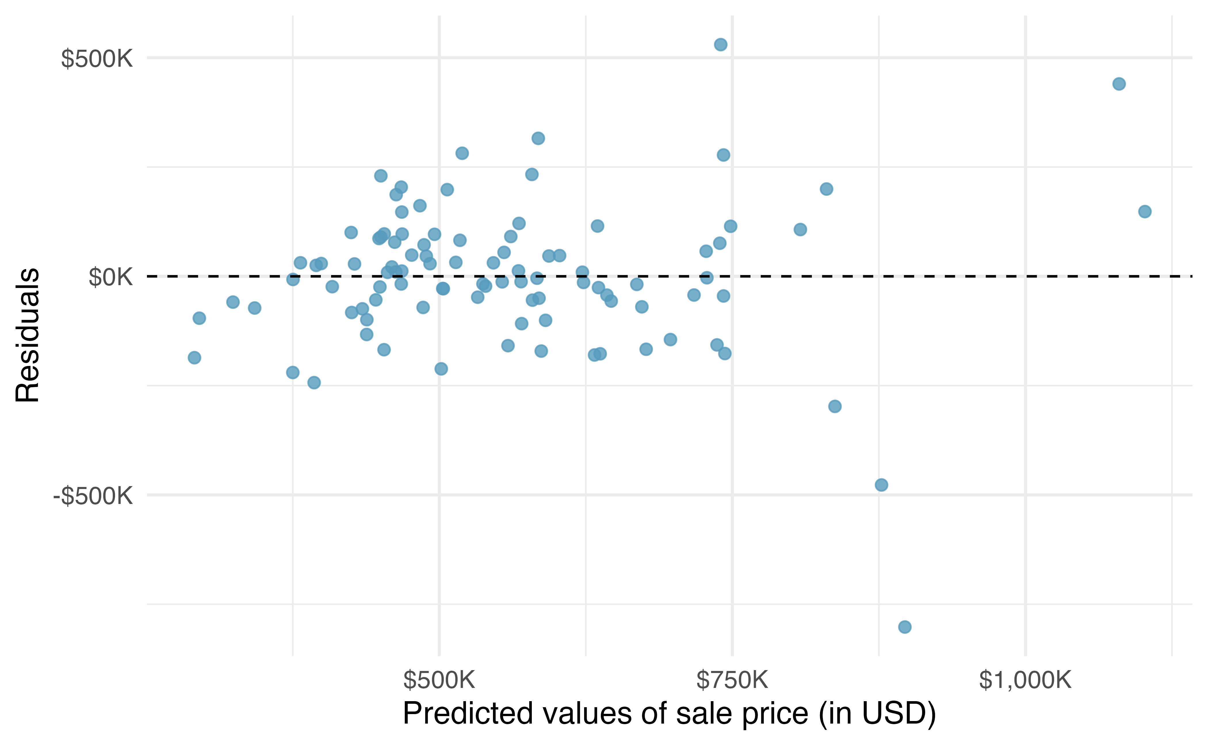
area and price of a home is indeed linear. However, the residuals are quite large for expensive homes. The large residuals indicate potential outliers or increasing variability, either of which could warrant more involved modeling techniques than are presented in this chapter.
price with multiple variables
price regressed on area, bed, bath, year_built, cooling, and lot.
| term | estimate | std.error | statistic | p.value |
|---|---|---|---|---|
(Intercept) |
-2,910,715 | 1,787,934 | -1.63 | 0.107 |
area |
102 | 23 | 4.42 | <0.0001 |
bed |
-13,692 | 25,928 | -0.53 | 0.5987 |
bath |
41,076 | 24,662 | 1.67 | 0.0993 |
year_built |
1,459 | 914 | 1.60 | 0.1139 |
coolingcentral |
84,065 | 30,338 | 2.77 | 0.0068 |
lot |
356,141 | 75,940 | 4.69 | <0.0001 |
| Adjusted R-sq = 0.5896 | ||||
| df = 90 | ||||
price. You consider taking a variable out, but you aren’t sure which one to remove.
area: 0.4846bed: 0.5609bath: 0.5488year_built: 0.4951cooling: 0.5423lot: 0.5051bed has the highest adjusted \(R^2\) of 0.5609, higher than the adjusted \(R^2\) for the full model. Because eliminating bed leads to a model with a higher adjusted \(R^2\) than the full model, we drop bed from the model. It might seem counter-intuitive to exclude number of bedrooms from the model. After all, we would expect homes with more bedrooms to cost more, and we can see a clear relationship between number of bedrooms and sale price in Figure 10.5. However, note that area is still in the model, and it’s quite likely that the area of the home and the number of bedrooms are highly associated. Therefore, the model already has information on "how much space is available in the house" with the inclusion of area.
bed:
bed and area: 0.4888bed and bath: 0.5526bed and year_built: 0.4972bed and cooling: 0.5440bed and lot: 0.5073bed, which we can summarize using the coefficients from Table 10.18.
| term | estimate | std.error | statistic | p.value |
|---|---|---|---|---|
(Intercept) |
-2,952,641 | 1,779,079 | -1.66 | 0.1004 |
area |
99 | 22 | 4.44 | <0.0001 |
bath |
36,228 | 22,799 | 1.59 | 0.1155 |
year_built |
1,466 | 910 | 1.61 | 0.1107 |
coolingcentral |
83,856 | 30,215 | 2.78 | 0.0067 |
lot |
357,119 | 75,617 | 4.72 | <0.0001 |
| Adjusted R-sq = 0.5929 | ||||
| df = 91 | ||||
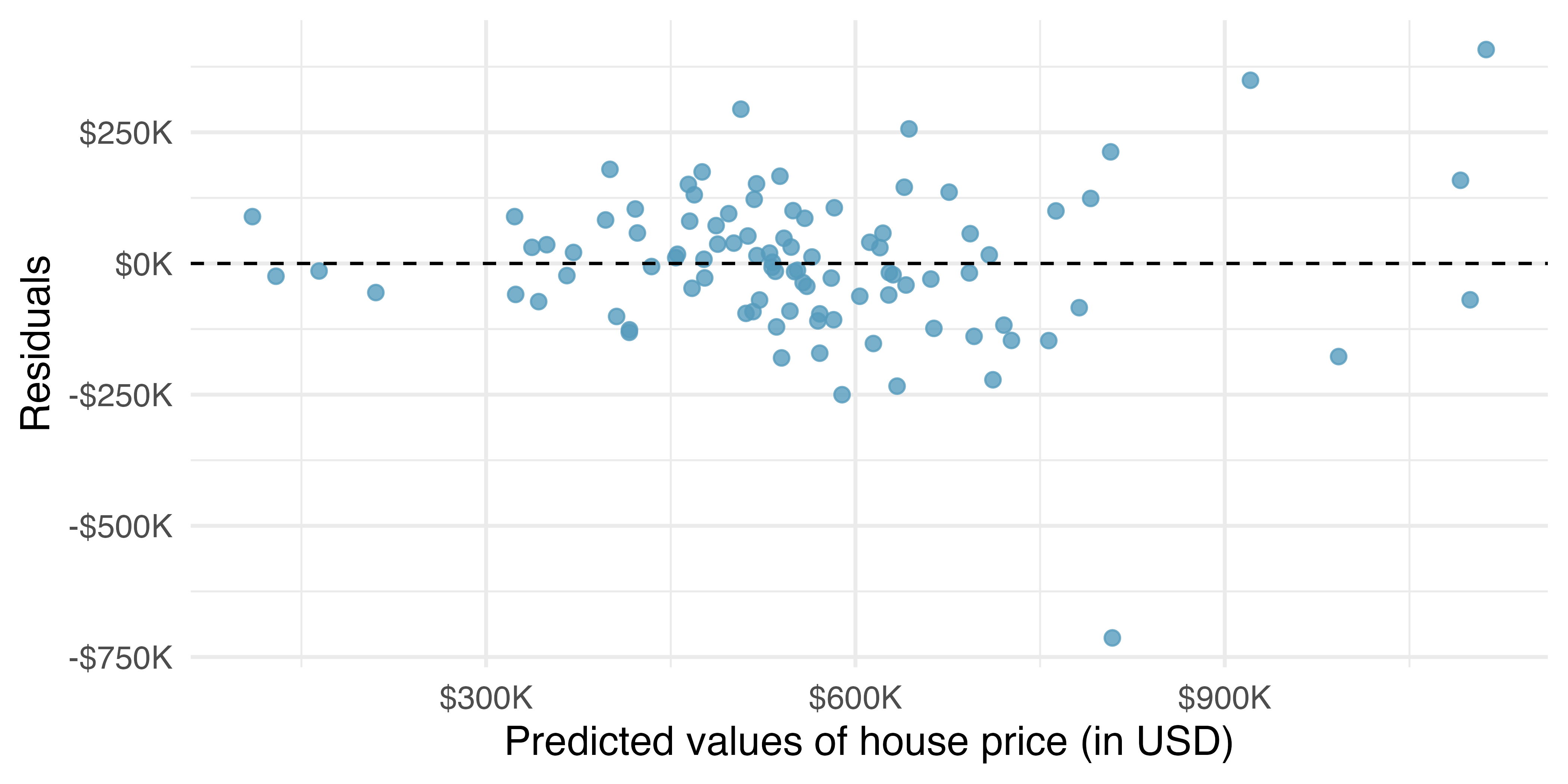
bed is given in Figure 10.21. How do the residuals in Figure 10.21 compare to the residuals in Figure 10.12?
m_full_no_bed |>
  augment() |>
  ggplot(aes(x = .fitted, y = .resid)) +
  geom_point(size = 2, alpha = 0.8) +
  labs(
    x = "Predicted values of house price (in USD)",
    y = "Residuals"
  ) +
  geom_hline(yintercept = 0, linetype = "dashed") +
  scale_x_continuous(labels = label_dollar(scale = 1/1000, suffix = "K")) +
  scale_y_continuous(labels = label_dollar(scale = 1/1000, suffix = "K"))