Inference for comparing paired means

Chapter 21 Inference for comparing paired means

In Chapter 20 analysis was done to compare the average population value across two different groups. Recall that one of the important conditions in doing a two-sample analysis is that the two groups are independent. Here, independence across groups means that knowledge of the observations in one group does not change what we would expect to happen in the other group. But what happens if the groups are dependent? Sometimes dependency is not something that can be addressed through a statistical method. However, a particular dependency, pairing, can be modeled quite effectively using many of the same tools we have already covered in this text.

🔗

Paired data represent a particular type of experimental structure where the analysis is somewhat akin to a one-sample analysis (see Chapter 19) but has other features that resemble a two-sample analysis (see Chapter 20). As with a two-sample analysis, quantitative measurements are made on each of two different levels of the explanatory variable. However, because the observational unit is paired across the two groups, the two measurements are subtracted such that only the difference is retained. Table 21.1 presents some examples of studies where paired designs were implemented.

🔗

Table 21.1. Examples of studies where a paired design is used to measure the difference in the measurement over two conditions

🔗

Listing 21.2. R code for tbl-pairedexamples

🔗

paired_study_examples <- tribble(
  ~variable, ~col1, ~col2, ~col3,
  "Car", "Smooth Turn vs Quick Spin", "amount of tire tread after 1,000 miles", "difference in tread",
  "Textbook", "UCLA vs Amazon", "price of new text", "difference in price",
  "Individual person", "Pre-course vs Post-course", "exam score", "difference in score"
)

paired_study_examples |>
  kbl(
    linesep = "", booktabs = TRUE,
    col.names = c("Observational unit", "Comparison groups", "Measurement", "Value of interest")
  ) |>
  kable_styling(
    bootstrap_options = c("striped", "condensed"),
    latex_options = c("striped"),
    full_width = FALSE
  ) |>
  column_spec(1:3, width = "8em")

Paired data.

Two sets of observations are paired if each observation in one set has a special correspondence or connection with exactly one observation in the other dataset.

🔗

It is worth noting that if mathematical modeling is chosen as the analysis tool, paired data inference on the difference in measurements will be identical to the one-sample mathematical techniques described in Chapter 19. However, recall from Chapter 19 that with pure one-sample data, the computational tools for hypothesis testing are not easy to implement and were not presented (although the bootstrap was presented as a computational approach for constructing a one sample confidence interval). With paired data, the randomization test fits nicely with the structure of the experiment and is presented here.

🔗

Section 21.1 Randomization test for the mean paired difference

Consider an experiment done to measure whether tire brand Smooth Turn or tire brand Quick Spin has longer tread wear (in cm). That is, after 1,000 miles on a car, which brand of tires has more tread, on average?

🔗

Subsection 21.1.1 Observed data

The observed data represent 25 tread measurements (in cm) taken on 25 tires of Smooth Turn and 25 tires of Quick Spin. The study used a total of 25 cars, so on each car, one tire was of Smooth Turn and one was of Quick Spin. The mean tread for the Quick Spin tires was 0.308 cm and the mean tread for the Smooth Turn tires was 0.310 cm. Figure 21.3 presents the observed data, calculations on tread remaining (in cm).

🔗

The Smooth Turn manufacturer looks at the box plots and says:

🔗

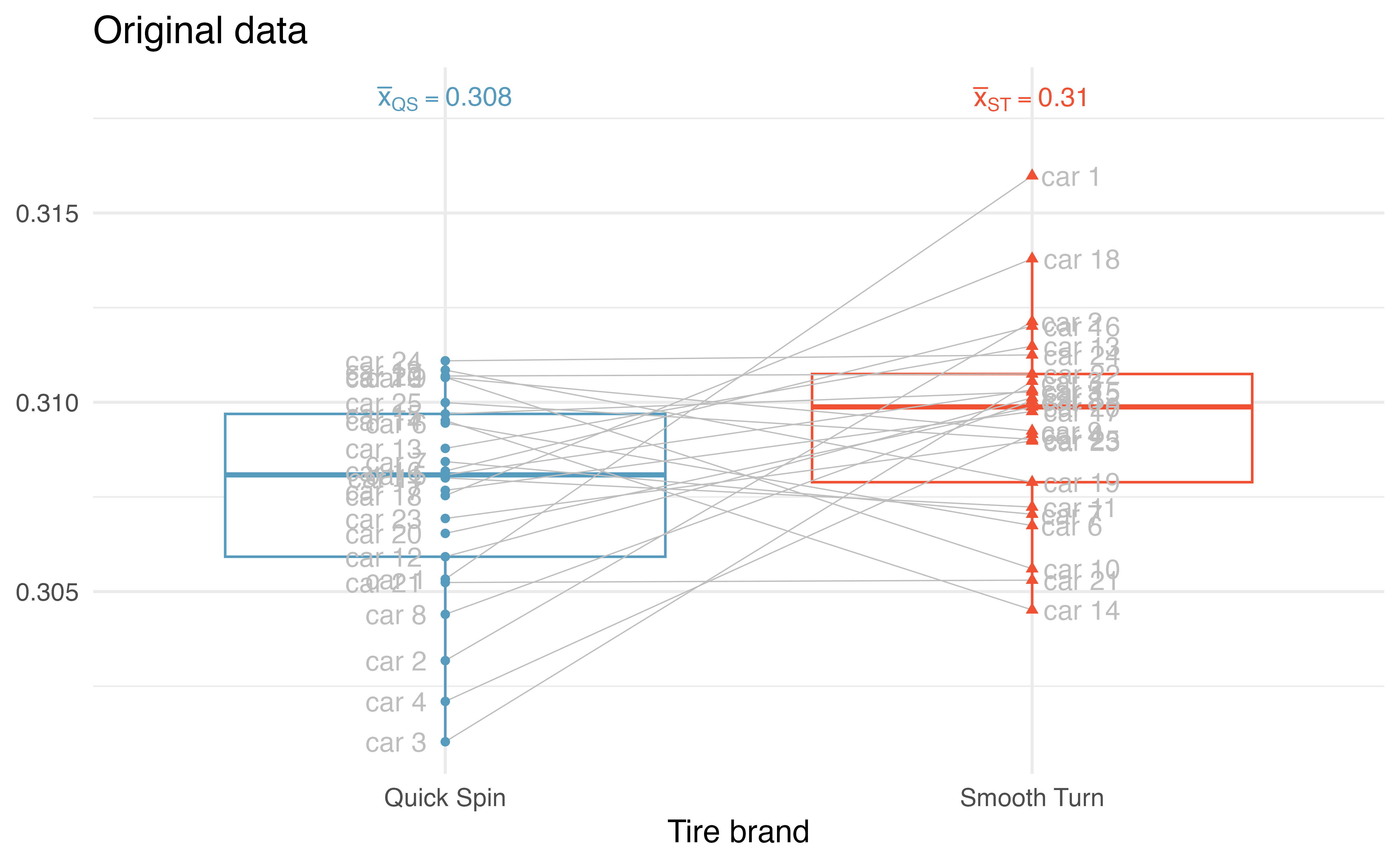
Clearly the tread on Smooth Turn tires is higher, on average, than the tread on Quick Spin tires after 1,000 miles of driving.
🔗

🔗

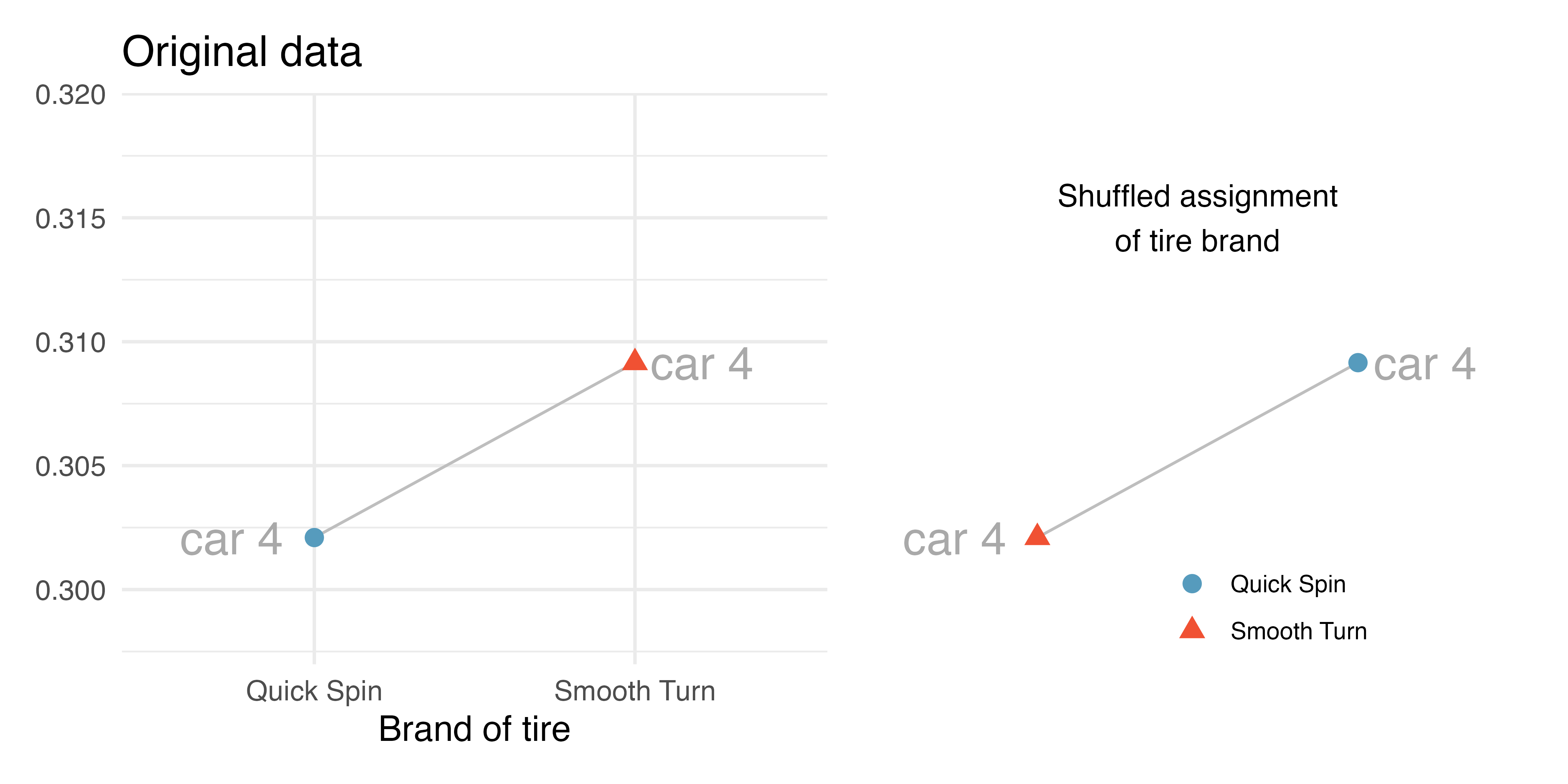
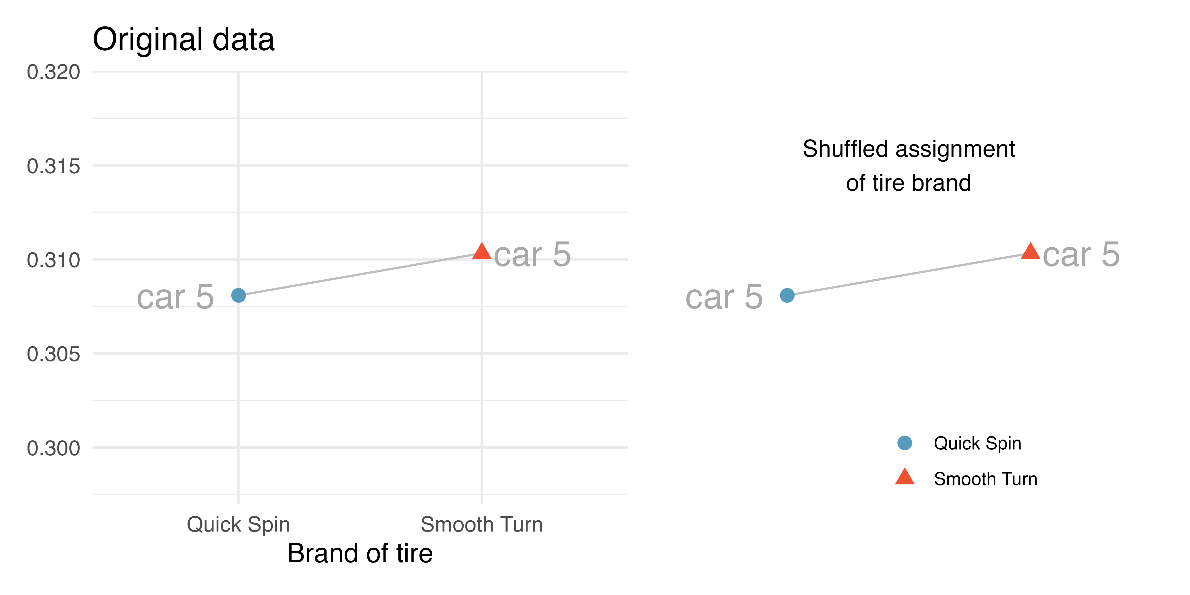
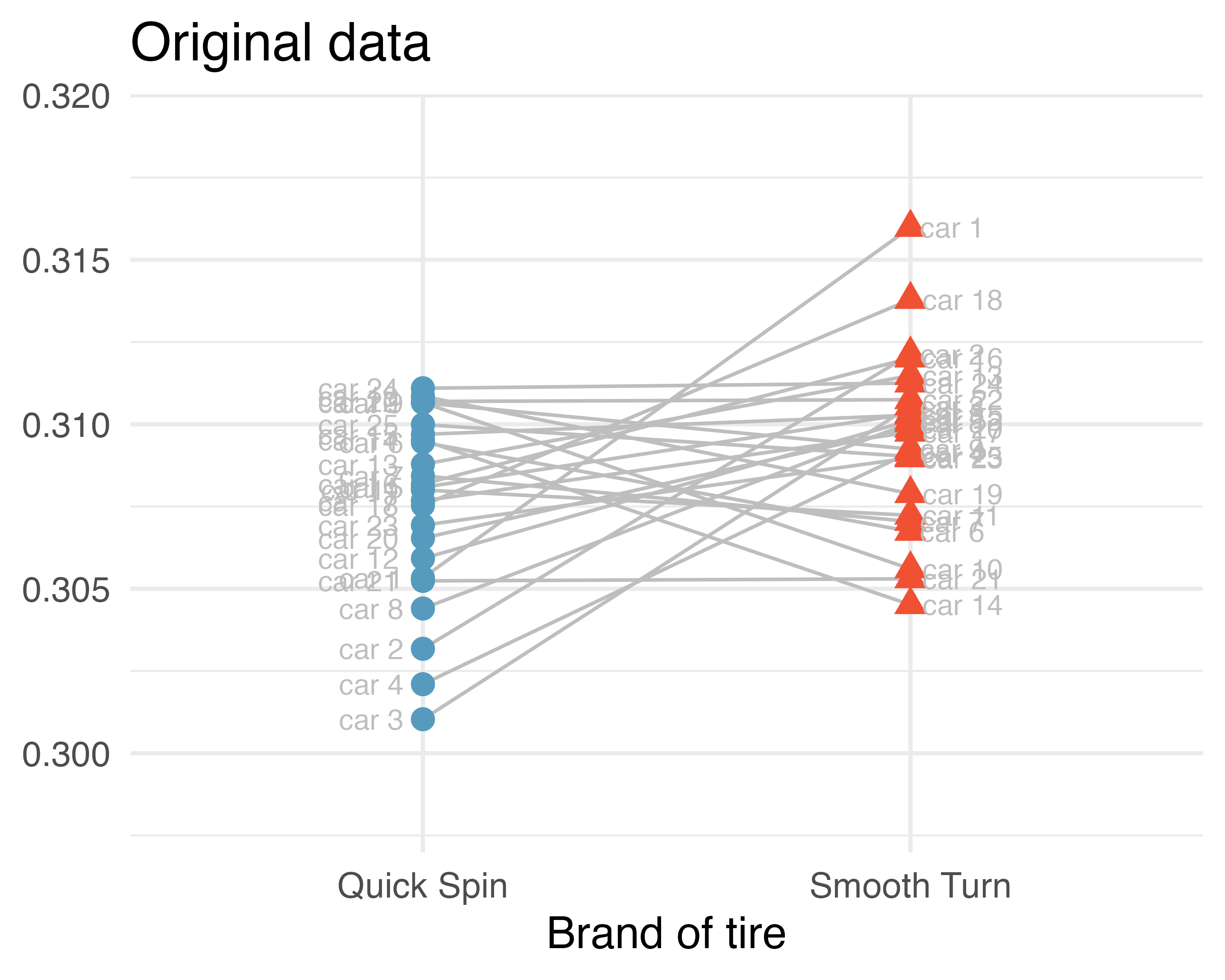
The Quick Spin manufacturer is skeptical and retorts:

🔗

But with only 25 cars, it seems that the variability in road conditions (sometimes one tire hits a pothole, etc.) could be what leads to the small difference in average tread amount.
🔗

🔗

Figure 21.3. Box plots of the tire tread data (in cm) and the brand of tire from which the original measurements came.
🔗

Listing 21.4. R code for fig-tiredata

🔗

set.seed(47)
brandA <- rnorm(25, 0.310, 0.003)
brandB <- rnorm(25, 0.308, 0.003)
car <- c(paste("car", 1:25))
miny <- min(brandA, brandB) - .003
maxy <- max(brandA, brandB) + .003

tires <- tibble(
  tread = c(brandA, brandB),
  car = rep(car, 2),
  brand = c(rep("Smooth Turn", 25), rep("Quick Spin", 25))
)

orig_means <- tires |>
  group_by(brand) |>
  summarize(mean_tread = round(mean(tread), 4)) |>
  mutate(
    mean_label = c("bar(x)[QS]", "bar(x)[ST]"),
    mean_label = paste(mean_label, "==", mean_tread)
  )

ggplot(tires, aes(
  x = brand, y = tread,
  color = brand, shape = brand
)) +
  geom_boxplot(
    show.legend = FALSE,
    outlier.shape = "triangle"
  ) +
  geom_text(aes(label = car),
    color = "grey",
    hjust = rep(c(-0.15, 1.3), each = 25),
    show.legend = FALSE, size = 4
  ) +
  geom_line(aes(group = car), color = "grey", linewidth = 0.25) +
  geom_point(show.legend = FALSE) +
  geom_text(
    data = orig_means,
    aes(label = mean_label, y = 0.318),
    parse = TRUE, show.legend = FALSE
  ) +
  scale_color_manual(values = c(IMSCOL["blue", "full"], IMSCOL["red", "full"])) +
  labs(
    x = "Tire brand",
    y = NULL,
    title = "Original data"
  )

We’d like to be able to systematically distinguish between what the Smooth Turn manufacturer sees in the plot and what the Quick Spin manufacturer sees in the plot. Fortunately for us, we have an excellent way to simulate the natural variability (from road conditions, etc.) that can lead to tires being worn at different rates.

🔗

Subsection 21.1.2 Variability of the statistic

A randomization test will identify whether the differences seen in the box plot of the original data in Figure 21.3 could have happened just by chance variability. As before, we will simulate the variability in the study under the assumption that the null hypothesis is true. In this study, the null hypothesis is that average tire tread wear is the same across Smooth Turn and Quick Spin tires.

🔗

$H_0: \mu_{diff} = 0,$ the average tread wear is the same for the two tire brands.
🔗

🔗
$H_A: \mu_{diff} \ne 0,$ the average tread wear is different across the two tire brands.
🔗

🔗

When observations are paired, the randomization process randomly assigns the tire brand to each of the observed tread values. Note that in the randomization test for the two-sample mean setting (see Section 20.1) the explanatory variable was also randomly assigned to the responses. The change in the paired setting, however, is that the assignment happens within an observational unit (here, a car). Remember, if the null hypothesis is true, it will not matter which brand is put on which tire because the overall tread wear will be the same across pairs.

🔗

Figure 21.5 and Figure 21.7 show that the random assignment of group (tire brand) happens within a single car. That is, every single car will still have one tire of each type. In the first randomization, it just so happens that the 4th car’s tire brands were swapped and the 5th car’s tire brands were not swapped.

🔗

Figure 21.5. The 4th car: the tire brand was randomly permuted, and in the randomization calculation, the measurements (in cm) ended up in different groups
🔗

Listing 21.6. R code for fig-tiredata4

🔗

set.seed(47)
permdata <- tires |>
  group_by(car) |>
  mutate(random_brand = sample(brand))

origplot4 <- tires |>
  filter(car == "car 4") |>
  ggplot(aes(
    x = brand, y = tread,
    color = brand, shape = brand
  )) +
  geom_line(aes(group = car), color = "grey") +
  geom_point(size = 3, show.legend = FALSE) +
  geom_text(aes(label = car),
    color = "darkgrey",
    hjust = rep(c(-0.15, 1.3), each = 1),
    show.legend = FALSE, size = 6
  ) +
  ylim(c(miny, maxy)) +
  labs(
    x = "Brand of tire",
    y = NULL,
    color = NULL, shape = NULL,
    title = "Original data"
  ) +
  scale_color_manual(values = c(IMSCOL["blue", "full"], IMSCOL["red", "full"]))

shuffbrand4 <- permdata |>
  filter(car == "car 4") |>
  ggplot(aes(
    x = brand, y = tread,
    color = random_brand, shape = random_brand
  )) +
  geom_line(aes(group = car), color = "grey") +
  geom_point(size = 3) +
  geom_text(aes(label = car),
    color = "darkgrey",
    hjust = rep(c(-0.15, 1.3), each = 1),
    show.legend = FALSE, size = 6
  ) +
  ylim(c(miny, maxy)) +
  scale_color_manual(values = c(IMSCOL["blue", "full"], IMSCOL["red", "full"])) +
  theme_void() +
  annotate(
    "text",
    x = 1.5, y = 0.315,
    label = "Shuffled assignment\nof tire brand",
    size = 4
  ) +
  theme(
    legend.position = c(0.6, 0.1),
    legend.background = element_rect(color = "white")
  ) +
  labs(color = NULL, shape = NULL)

origplot4 + shuffbrand4

Figure 21.7. The 5th car: the tire brand was randomly permuted to stay the same! In the randomization calculation, the measurements (in cm) ended up in the original groups
🔗

Listing 21.8. R code for fig-tiredata5

🔗

origplot5 <- tires |>
  filter(car == "car 5") |>
  ggplot(aes(
    x = brand, y = tread,
    color = brand, shape = brand
  )) +
  geom_line(aes(group = car), color = "grey") +
  geom_point(size = 3, show.legend = FALSE) +
  geom_text(aes(label = car),
    color = "darkgrey",
    hjust = rep(c(-0.15, 1.3), each = 1),
    show.legend = FALSE, size = 6
  ) +
  ylim(c(miny, maxy)) +
  labs(
    x = "Brand of tire",
    y = NULL,
    color = NULL, shape = NULL,
    title = "Original data"
  ) +
  scale_color_manual(values = c(IMSCOL["blue", "full"], IMSCOL["red", "full"]))

shuffbrand5 <- permdata |>
  filter(car == "car 5") |>
  ggplot(aes(
    x = brand, y = tread,
    color = random_brand, shape = random_brand
  )) +
  geom_line(aes(group = car), color = "grey") +
  geom_point(size = 3) +
  geom_text(aes(label = car),
    color = "darkgrey",
    hjust = rep(c(-0.15, 1.3), each = 1),
    show.legend = FALSE, size = 6
  ) +
  ylim(c(miny, maxy)) +
  scale_color_manual(values = c(IMSCOL["blue", "full"], IMSCOL["red", "full"])) +
  theme_void() +
  annotate(
    "text",
    x = 1.5, y = 0.315,
    label = "Shuffled assignment\nof tire brand",
    size = 4
  ) +
  theme(
    legend.position = c(0.6, 0.1),
    legend.background = element_rect(color = "white")
  ) +
  labs(color = NULL, shape = NULL)

origplot5 + shuffbrand5

We can put the shuffled assignments for all the cars into one plot as seen in Figure 21.9.

🔗

Figure 21.9. Tire tread (in cm) by brand, original and shuffled. As evidenced by the colors, some of the cars kept their original tire assignments and some cars swapped the tire assignments.
🔗

Listing 21.10. R code for fig-tiredataPerm

🔗

origplot <- tires |>
  ggplot(aes(
    x = brand, y = tread,
    color = brand, shape = brand
  )) +
  geom_line(aes(group = car), color = "grey") +
  geom_point(size = 3, show.legend = FALSE) +
  geom_text(aes(label = car),
    color = "grey",
    hjust = rep(c(-0.15, 1.3), each = nrow(tires) / 2),
    show.legend = FALSE, size = 3
  ) +
  ylim(c(miny, maxy)) +
  labs(
    x = "Brand of tire",
    y = NULL,
    color = NULL, shape = NULL,
    title = "Original data"
  ) +
  scale_color_manual(values = c(IMSCOL["blue", "full"], IMSCOL["red", "full"]))

shuffbrand <- permdata |>
  ggplot(aes(
    x = brand, y = tread,
    color = random_brand, shape = random_brand
  )) +
  geom_line(aes(group = car), color = "grey") +
  geom_point(size = 3) +
  geom_text(aes(label = car),
    color = "grey",
    hjust = rep(c(-0.15, 1.3), each = nrow(tires) / 2),
    show.legend = FALSE, size = 3
  ) +
  ylim(c(miny, maxy)) +
  scale_color_manual(values = c(IMSCOL["blue", "full"], IMSCOL["red", "full"])) +
  theme_void() +
  theme(
    legend.position = c(0.6, 0.1),
    legend.background = element_rect(color = "white")
  ) +
  labs(
    title = "Shuffled data",
    color = NULL, shape = NULL
  )

origplot
shuffbrand

The next step in the randomization test is to sort the brands so that the assigned brand value on the x-axis aligns with the assigned group from the randomization. Figure 21.11 shows the same randomized groups, as seen in Figure 21.9 previously. However, Figure 21.11 sorts the randomized groups so that we can measure the variability across groups as compared to the variability within groups.

🔗

Figure 21.11. Tire tread (in cm) by brand.
🔗

Listing 21.12. R code for fig-tiredataPermSort

🔗

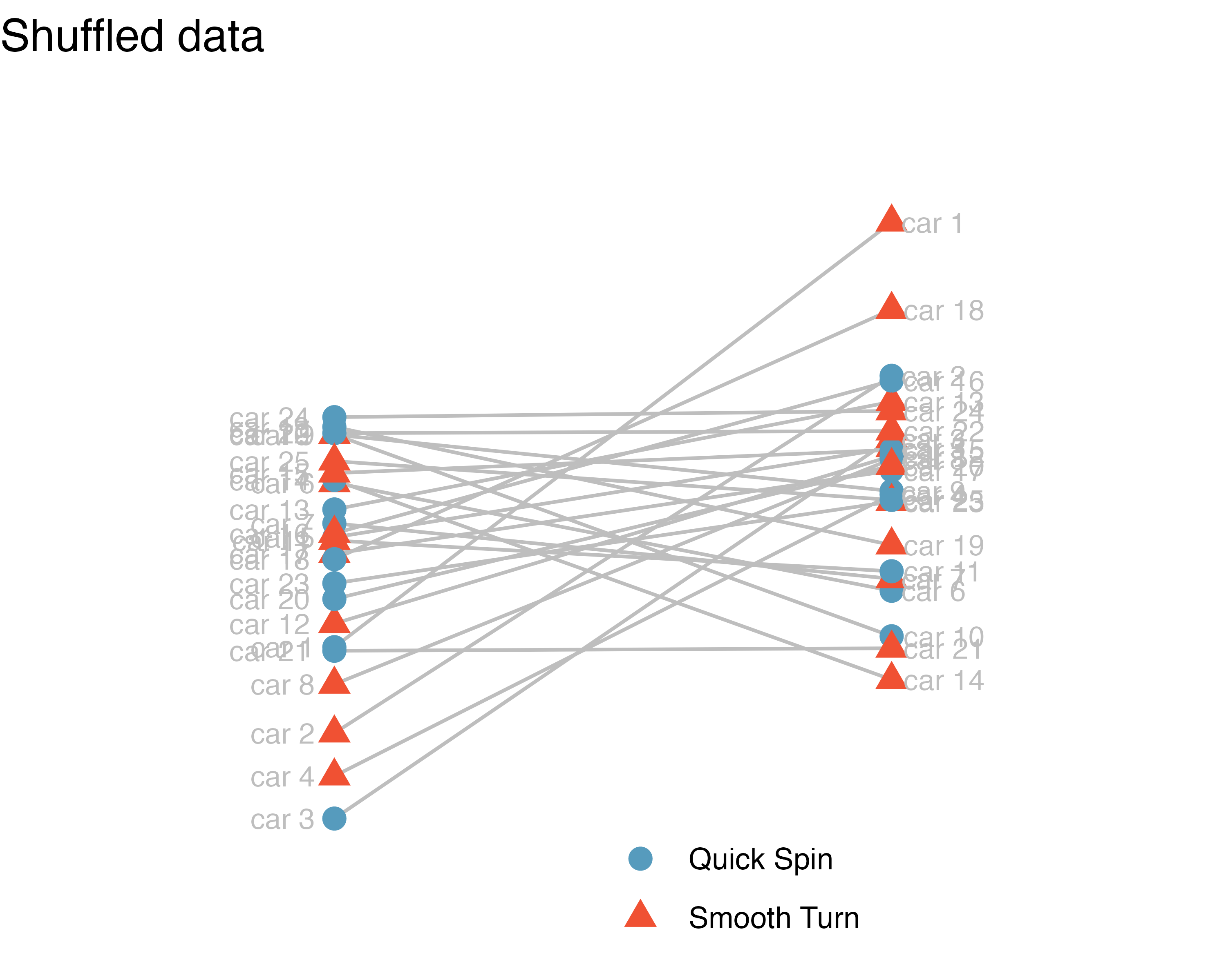
permed_means <- permdata |>
  group_by(random_brand) |>
  summarize(mean_tread = round(mean(tread), 4)) |>
  mutate(mean_label = c("bar(x)[QSsim1]", "bar(x)[STsim1]")) |>
  mutate(mean_label = paste(mean_label, "==", mean_tread))

shuffbrandfull <- permdata |>
  ggplot(aes(
    x = random_brand, y = tread,
    color = random_brand, shape = random_brand
  )) +
  geom_text(aes(label = car),
    color = "grey",
    hjust = rep(c(-0.15, 1.3), each = 25),
    show.legend = FALSE, size = 3
  ) +
  geom_line(aes(group = car), color = "grey") +
  ylim(c(miny, maxy)) +
  geom_point(size = 3, show.legend = FALSE) +
  geom_text(
    data = permed_means,
    aes(label = mean_label, y = 0.318),
    parse = TRUE, show.legend = FALSE
  ) +
  labs(
    x = "Randomized brand of tire",
    y = NULL,
    title = "Sorted data"
  ) +
  scale_color_manual(values = c(IMSCOL["blue", "full"], IMSCOL["red", "full"]))

shuffbrand
shuffbrandfull

Figure 21.13 presents a second randomization of the data. Notice that the two observations from the same car are linked with a grey line; some of the tread values have been randomly assigned to the other tire brand, while some are still connected to their original tire brands.

🔗

Figure 21.13. A second randomization where the brand is randomly swapped (or not) across the two tread wear measurements (in cm) from the same car.
🔗

Listing 21.14. R code for fig-tiredatarand1

🔗

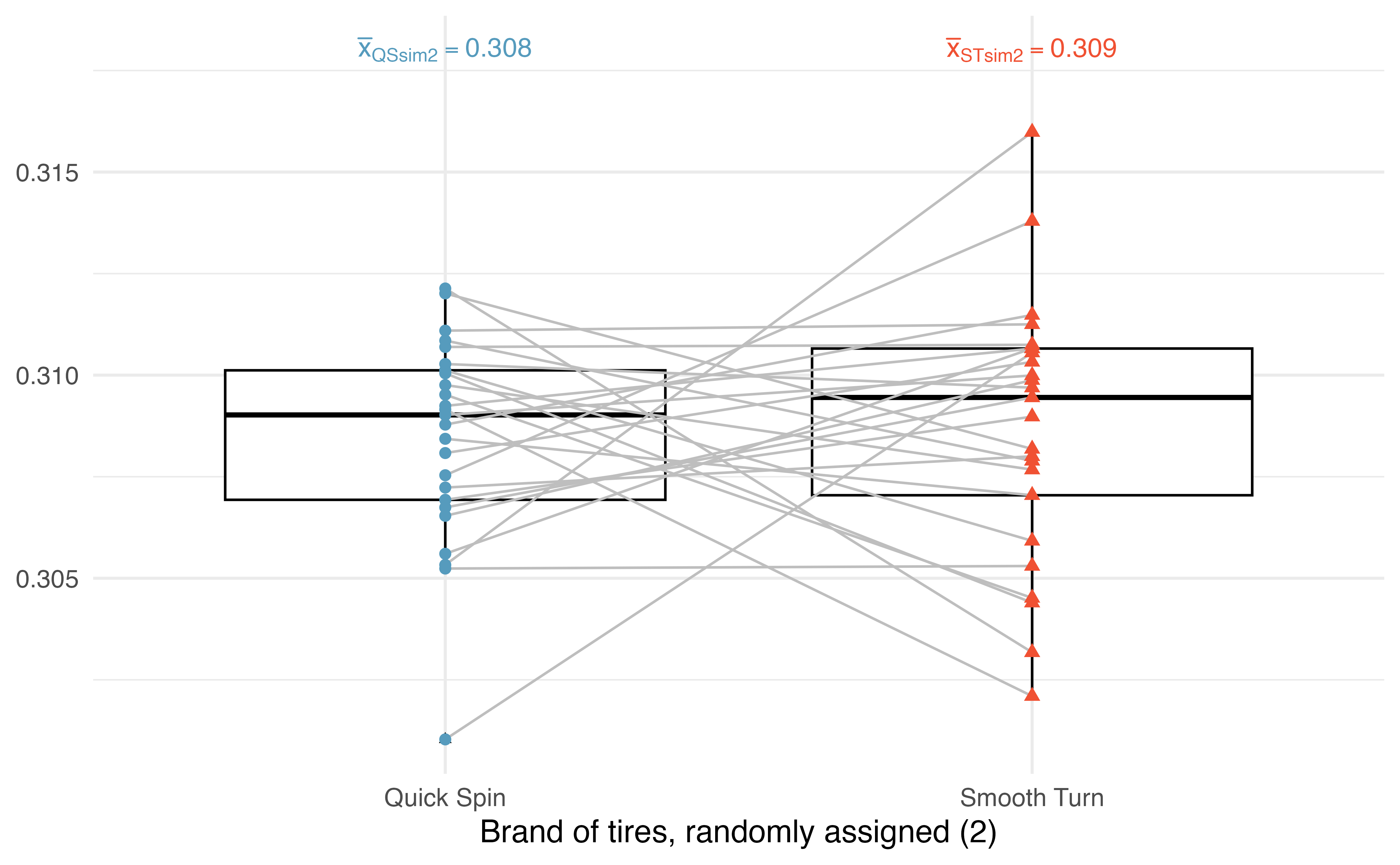
set.seed(47)
tires1 <- tires |>
  group_by(car) |>
  mutate(random_brand = sample(brand))

permed_means <- tires1 |>
  group_by(random_brand) |>
  summarize(mean_tread = round(mean(tread), 4)) |>
  mutate(mean_label = c("bar(x)[QSsim2]", "bar(x)[STsim2]")) |>
  mutate(mean_label = paste(mean_label, "==", mean_tread))

ggplot(
  tires1, aes(
    x = random_brand, y = tread,
    color = random_brand, shape = random_brand
  )
) +
  geom_boxplot(
    show.legend = FALSE, color = "black",
    outlier.shape = "triangle"
  ) +
  geom_line(aes(group = car), color = "grey") +
  geom_point(size = 2, show.legend = FALSE) +
  geom_text(
    data = permed_means,
    aes(label = mean_label, y = 0.318),
    parse = TRUE, show.legend = FALSE
  ) +
  scale_color_manual(values = c(IMSCOL["blue", "full"], IMSCOL["red", "full"])) +
  labs(
    x = "Brand of tires, randomly assigned (2)",
    y = NULL
  )

Figure 21.15 presents yet another randomization of the data. Again, the same observations are linked by a grey line, and some of the tread values have been randomly assigned to the opposite tire brand than they were originally (while some are still connected to their original tire brands).

🔗

Figure 21.15. An additional randomization where the brand is randomly swapped (or not) across the two tread wear measurements (in cm) from the same car.
🔗

Listing 21.16. R code for fig-tiredatarand2

🔗

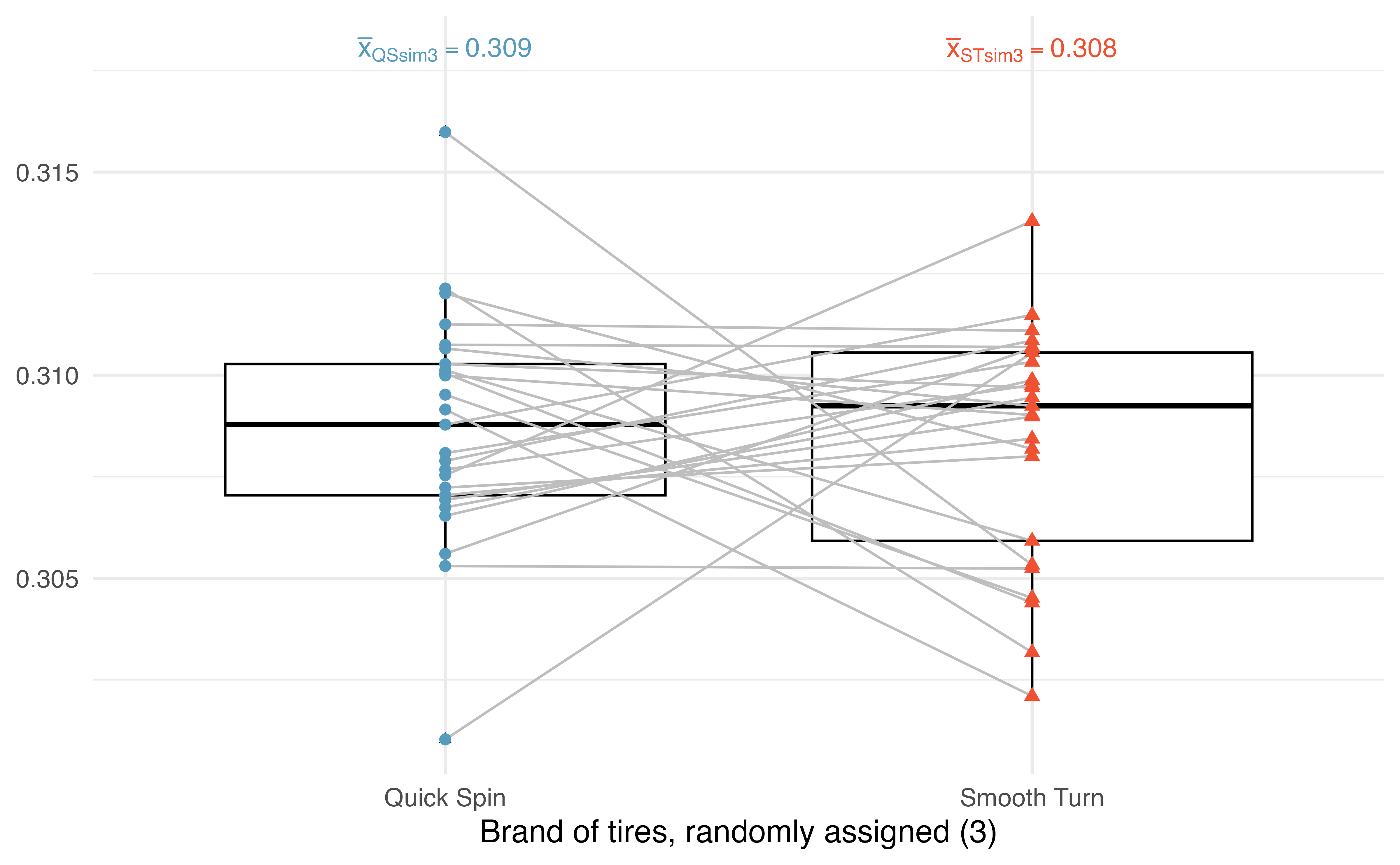
set.seed(4747)
tires2 <- tires |>
  group_by(car) |>
  mutate(random_brand = sample(brand))

permed_means <- tires2 |>
  group_by(random_brand) |>
  summarize(mean_tread = round(mean(tread), 4)) |>
  mutate(mean_label = c("bar(x)[QSsim3]", "bar(x)[STsim3]")) |>
  mutate(mean_label = paste(mean_label, "==", mean_tread))

ggplot(
  tires2,
  aes(
    x = random_brand, y = tread,
    color = random_brand, shape = random_brand
  )
) +
  geom_boxplot(
    show.legend = FALSE, color = "black",
    outlier.shape = "triangle"
  ) +
  geom_line(aes(group = car), color = "grey") +
  geom_point(size = 2, show.legend = FALSE) +
  geom_text(
    data = permed_means,
    aes(label = mean_label, y = 0.318),
    parse = TRUE, show.legend = FALSE
  ) +
  scale_color_manual(values = c(IMSCOL["blue", "full"], IMSCOL["red", "full"])) +
  labs(
    x = "Brand of tires, randomly assigned (3)",
    y = NULL
  )

🔗

Subsection 21.1.3 Observed statistic vs. null statistics

By repeating the randomization process, we can create a distribution of the average of the differences in tire treads, as seen in Figure 21.17. As expected (because the differences were generated under the null hypothesis), the center of the histogram is zero. A line has been drawn at the observed difference which is well outside the majority of the null differences simulated from natural variability by mixing up which the tire received Smooth Turn and which received Quick Spin. Because the observed statistic is so far away from the natural variability of the randomized differences, we are convinced that there is a difference between Smooth Turn and Quick Spin. Our conclusion is that the extra amount of average tire tread in Smooth Turn is due to more than just natural variability: we reject $H_0$ and conclude that $\mu_{ST} \ne \mu_{QS}.$

🔗

Figure 21.17. Histogram of 1,000 mean differences with tire brand randomly assigned across the two tread measurements (in cm) per pair.
🔗

Listing 21.18. R code for fig-pair-randomize

🔗

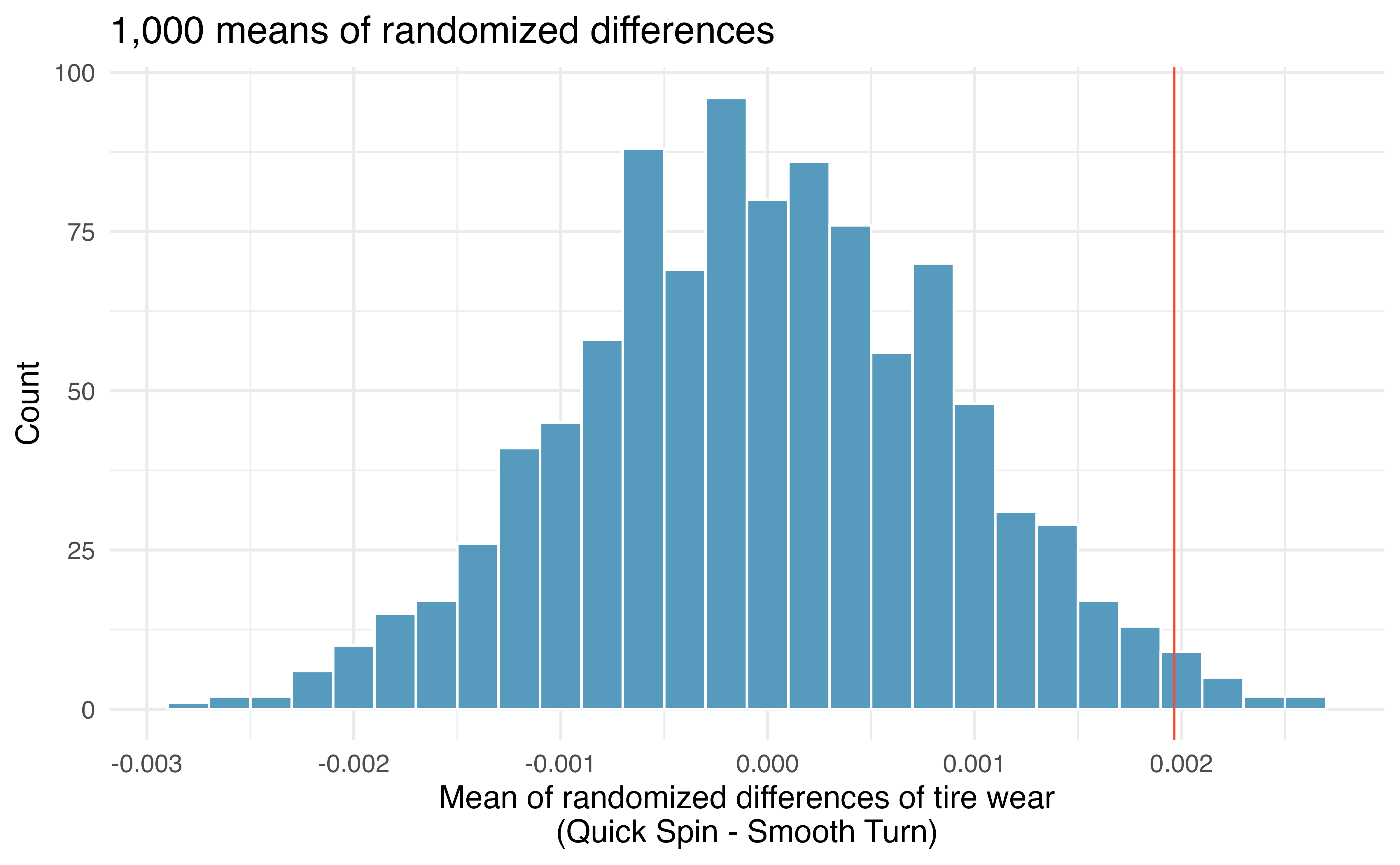
set.seed(474756)
tires_shuffled <- tires |>
  pivot_wider(
    id_cols = car, names_from = brand, names_prefix = "brand_",
    values_from = tread
  ) |>
  mutate(diff_tread = `brand_Quick Spin` - `brand_Smooth Turn`) |>
  specify(response = diff_tread) |>
  hypothesize(null = "paired independence") |>
  generate(1000, type = "permute") |>
  calculate(stat = "mean")

ggplot(tires_shuffled, aes(x = stat)) +
  geom_histogram(binwidth = 0.0002) +
  labs(
    x = "Mean of randomized differences of tire wear\n(Quick Spin - Smooth Turn)",
    title = "1,000 means of randomized differences",
    y = "Count"
  ) +
  geom_vline(
    xintercept = mean(brandA) - mean(brandB),
    color = IMSCOL["red", "full"]
  )

🔗

Section 21.2 Bootstrap confidence interval for the mean paired difference

For both the bootstrap and the mathematical models applied to paired data, the analysis is virtually identical to the one-sample approach given in Chapter 19. The key to working with paired data (for bootstrapping and mathematical approaches) is to consider the measurement of interest to be the difference in measured values across the pair of observations.

🔗

Subsection 21.2.1 Observed data

In an earlier edition of this textbook, we found that Amazon prices were, on average, lower than those of the UCLA Bookstore for UCLA courses in 2010. It’s been several years, and many stores have adapted to the online market, so we wondered, how is the UCLA Bookstore doing today?

🔗

We sampled 201 UCLA courses. Of those, 68 required books could be found on Amazon, where prices are in US dollars.

🔗

Note 21.19. Data.

The ucla_textbooks_f18 data can be found in the openintro R package.

🔗

Table 21.20. Four cases from the ucla_textbooks_f18 dataset

🔗

subject	course_num	bookstore_new	amazon_new	price_diff
American Indian Studies	M10	48.0	47.5	0.52
Anthropology	2	14.3	13.6	0.71
Arts and Architecture	10	13.5	12.5	0.97
Asian	M60W	49.3	55.0	-5.69

Listing 21.21. R code for tbl-textbooksDF

🔗

ucla_textbooks_f18 |>
  select(subject, course_num, bookstore_new, amazon_new) |>
  mutate(price_diff = bookstore_new - amazon_new) |>
  filter(!is.na(bookstore_new) & !is.na(amazon_new)) |>
  head(4) |>
  kbl(linesep = "", booktabs = TRUE) |>
  kable_styling(
    bootstrap_options = c("striped", "condensed"),
    latex_options = c("striped"), full_width = FALSE
  )

Each textbook has two corresponding prices in the dataset: one for the UCLA Bookstore and one for Amazon. When two sets of observations have this special correspondence, they are said to be paired.

🔗

Subsection 21.2.2 Variability of the statistic

Following the example of bootstrapping the one-sample statistic, the observed differences can be bootstrapped in order to understand the variability of the average difference from sample to sample. Remember, the differences act as a single value to bootstrap. That is, the original dataset would include the list of 68 price differences, and each resample will also include 68 price differences (some repeated through the bootstrap resampling process). The bootstrap procedure for paired differences is quite similar to the procedure applied to the one-sample statistic case in Section 19.1.

🔗

In Figure 21.23, two 99% confidence intervals for the difference in the cost of a new book at the UCLA bookstore compared with Amazon have been calculated. The bootstrap percentile confidence interval is computed using the 0.5 percentile and 99.5 percentile bootstrapped differences and is found to be ($\$0.25, \$7.87$).

🔗

Checkpoint 21.22. Checkpoint.

Using the histogram of bootstrapped difference in means, estimate the standard error of the mean of the sample differences, $\bar{x}_{diff}.$

🔗

Using the histogram of bootstrapped difference in means, estimate the standard error of the mean of the sample differences, $\bar{x}_{diff}.$

🔗

Solution.

The bootstrapped differences in sample means vary roughly from 0.7 to 7.5, a range of \$6.80.

🔗

Although the bootstrap distribution is not symmetric, we use the empirical rule (that with bell-shaped distributions, most observations are within two standard errors of the center), the standard error of the mean differences is approximately \$1.70.

🔗

You might note that the standard error calculation given in Section 21.3 is $SE(\bar{x}_{diff}) = \sqrt{s^2_{diff}/n_{diff}} = \sqrt{13.4^2/68} = \$1.62$ (values from Section 21.3), very close to the bootstrap approximation.

🔗

The bootstrap SE interval is found by computing the SE of the bootstrapped differences $SE_{\overline{x}_{diff}} = \$1.64$ and the normal multiplier of $z^{\star} = 2.58.$ The averaged difference is $\bar{x} = \$3.58.$ The 99% confidence interval is: $\$3.58 \pm 2.58 \times \$1.64 = (\$-0.65, \$7.81).$

🔗

The confidence intervals seem to indicate that the UCLA bookstore price is, on average, higher than the Amazon price, as the majority of the confidence interval is positive. However, if the analysis required a strong degree of certainty (e.g., 99% confidence), and the bootstrap SE interval was most appropriate (given a second course in statistics the nuances of the methods can be investigated), the results of which bookseller is higher are not well determined (because the bootstrap SE interval overlaps zero). That is, the 99% bootstrap SE interval gives potential for UCLA bookstore to be lower, on average, than Amazon (because of the possible negative values for the true mean difference in price).

🔗

Figure 21.23. Bootstrap distribution for the average difference in new book price at the UCLA bookstore versus Amazon. 99% confidence intervals are superimposed using blue dashed (bootstrap percentile interval) and red dotted (bootstrap SE interval) lines.
🔗

Listing 21.24. R code for fig-pairboot

🔗

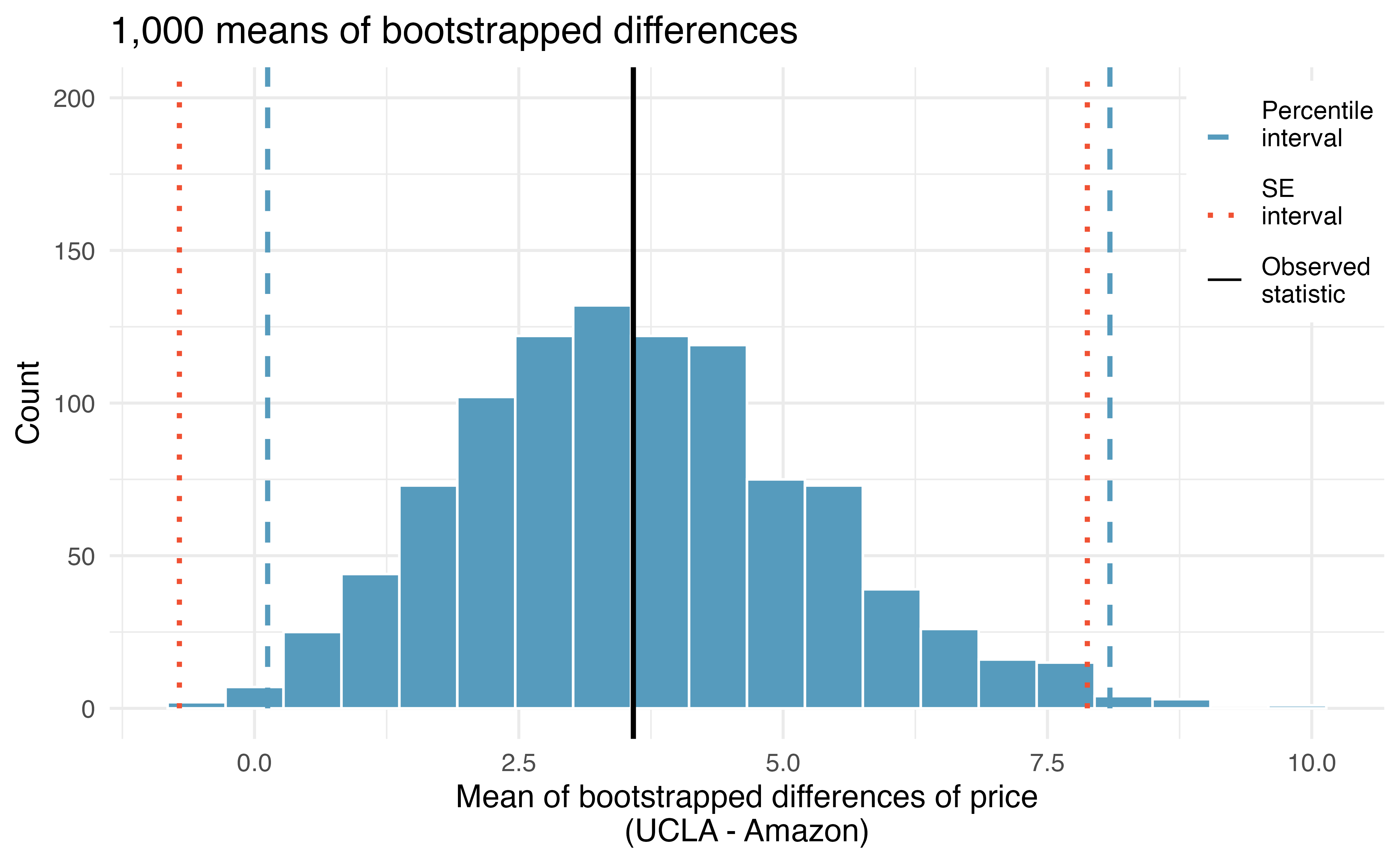
diff_price <- ucla_textbooks_f18 |>
  select(subject, course_num, bookstore_new, amazon_new) |>
  mutate(price_diff = bookstore_new - amazon_new) |>
  filter(!is.na(bookstore_new) & !is.na(amazon_new)) |>
  specify(response = price_diff) |>
  calculate(stat = "mean")

boot_diff <- ucla_textbooks_f18 |>
  select(subject, course_num, bookstore_new, amazon_new) |>
  mutate(price_diff = bookstore_new - amazon_new) |>
  filter(!is.na(bookstore_new) & !is.na(amazon_new)) |>
  specify(response = price_diff) |>
  generate(reps = 1000, type = "bootstrap") |>
  calculate(stat = "mean")

ci_perc_diff <- boot_diff |>
  get_confidence_interval(level = 0.99, type = "percentile")

ci_se_diff <- boot_diff |>
  get_confidence_interval(
    level = 0.99, type = "se",
    point_estimate = diff_price
  )

boot_diff |>
  infer::visualize(bins = 20) +
  infer::shade_confidence_interval(ci_perc_diff,
    color = IMSCOL["blue", "full"],
    fill = NULL, linewidth = 1, linetype = "dashed"
  ) +
  infer::shade_confidence_interval(ci_se_diff,
    color = IMSCOL["red", "full"],
    fill = NULL, linewidth = 1, linetype = "dotted"
  ) +
  geom_vline(xintercept = diff_price$stat, linewidth = 1) +
  geom_line(aes(y = replicate, x = stat, color = "a", linetype = "a"), alpha = 0, linewidth = 1) + # bogus code
  geom_line(aes(y = replicate, x = stat, color = "b", linetype = "b"), alpha = 0, linewidth = 1) + # bogus code
  geom_line(aes(y = replicate, x = stat, color = "c", linetype = "c"), alpha = 0) + # bogus code
  ylim(c(0, 200)) +
  guides(color = guide_legend(override.aes = list(alpha = 1))) +
  scale_color_manual(
    name = NULL,
    values = c("a" = IMSCOL["blue", "full"], "b" = IMSCOL["red", "full"], "c" = IMSCOL["black", "full"]),
    labels = c("Percentile\ninterval\n", "SE\ninterval\n", "Observed\nstatistic"),
    guide = "legend"
  ) +
  scale_linetype_manual(
    name = NULL,
    values = c("a" = "dashed", "b" = "dotted", "c" = "solid"),
    labels = c("Percentile\ninterval\n", "SE\ninterval\n", "Observed\nstatistic"),
    guide = "legend"
  ) +
  labs(
    x = "Mean of bootstrapped differences of price\n(UCLA - Amazon)",
    title = "1,000 means of bootstrapped differences",
    y = "Count"
  ) +
  theme(
    legend.position = c(0.925, 0.8),
    legend.background = element_rect(color = "white")
  )

🔗

Section 21.3 Mathematical model for the mean paired difference

Thinking about the differences as a single observation on an observational unit changes the paired setting into the one-sample setting. The mathematical model for the one-sample case is covered in Section 19.2.

🔗

Subsection 21.3.1 Observed data

To analyze paired data, it is often useful to look at the difference in outcomes of each pair of observations. In the textbook data, we look at the differences in prices, which is represented as the price_difference variable in the dataset. Here the differences are taken as:

🔗

UCLA Bookstore Price - Amazon price

🔗

It is important that we always subtract using a consistent order; here Amazon prices are always subtracted from UCLA prices. The first difference is shown in Table 21.20 and computed as $47.97-47.45=0.52\text{.}$ Similarly, the second difference is computed as $14.26-13.55=0.71\text{,}$ and the third is $13.50-12.53 = 0.97$ A histogram of the differences is shown in Figure 21.25

🔗

Figure 21.25. Histogram of the differences in prices for each book sampled.
🔗

🔗

Subsection 21.3.2 Variability of the statistic

To analyze a paired dataset, we simply analyze the differences. Table 21.26 provides the data summaries from the textbook data. Note that instead of reporting the prices separately for UCLA and Amazon, the summary statistics are given by the mean of the differences, the standard deviation of the differences, and the total number of pairs (i.e., differences). The parameter of interest is also a single value, $\mu_{diff},$ so we can use the same $t$-distribution techniques we applied in Section 19.2 directly onto the observed differences.

🔗

Table 21.26. Summary statistics for the 68 price differences

🔗

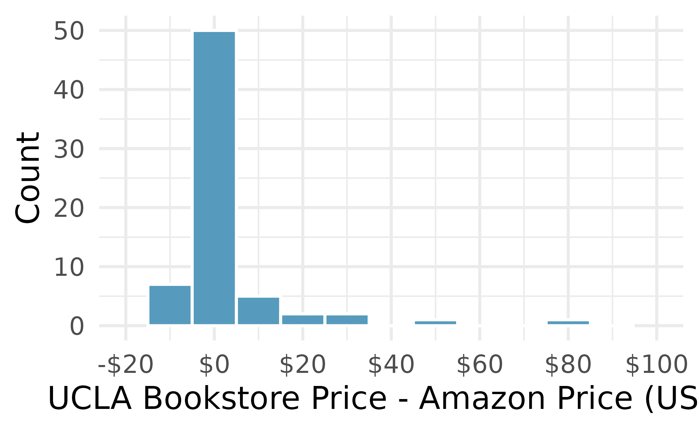
n	Mean	SD
68	3.58	13.4

Listing 21.27. R code for tbl-textbooksSummaryStats

🔗

ucla_textbooks_f18 |>
  summarise(
    n = n(),
    mean = mean(price_diff),
    sd = sd(price_diff)
  ) |>
  kbl(
    linesep = "", booktabs = TRUE,
    col.names = c("n", "Mean", "SD"),
    align = "ccc", digits = 2
  ) |>
  kable_styling(
    bootstrap_options = c("striped", "condensed"),
    latex_options = c("striped"), full_width = FALSE
  ) |>
  column_spec(1, width = "8em") |>
  column_spec(2, width = "8em") |>
  column_spec(3, width = "8em")

Example 21.28.

Set up a hypothesis test to determine whether, on average, there is a difference between Amazon’s price for a book and the UCLA bookstore’s price.

🔗

Also, check the conditions for whether we can move forward with the test using the $t$-distribution.

🔗

------------------------------------------------------------------------

🔗

We are considering two scenarios:

🔗

- $H_0:$ $\mu_{diff} = 0.$ There is no difference in the average textbook prices.

🔗

- $H_A:$ $\mu_{diff} \neq 0.$ There is a difference in average prices.

🔗

Next, we check the independence and normality conditions.

🔗

This is a simple random sample, so assuming the textbooks are independent seems reasonable.

🔗

While there are some outliers, $n = 68$ and none of the outliers are particularly extreme, so the normality of $\bar{x}$ is satisfied.

🔗

With these conditions satisfied, we can move forward with the $t$-distribution.

🔗

Subsection 21.3.3 Observed statistic vs. null statistics

As mentioned previously, the methods applied to a difference will be identical to the one-sample techniques. Therefore, the full hypothesis test framework is presented as guided practices.

🔗

The test statistic for assessing a paired mean is a T..

The T score is a ratio of how the sample mean difference varies from zero as compared to how the observations vary.

🔗

$T = \frac{\bar{x}_{diff} - 0 }{s_{diff}/\sqrt{n_{diff}}}$

🔗

When the null hypothesis is true and the conditions are met, T has a t-distribution with $df = n_{diff} - 1.$

🔗

Conditions:

🔗

- Independently sampled pairs.

🔗

- Large samples and no extreme outliers.

🔗

Example 21.29.

Complete the hypothesis test started in the previous Example.

🔗

------------------------------------------------------------------------

🔗

To compute the test compute the standard error associated with $\bar{x}_{diff}$ using the standard deviation of the differences $(s_{diff} = 13.42)$ and the number of differences $(n_{diff} = 68):$

🔗

$$SE_{\bar{x}_{diff}} = \frac{s_{diff}}{\sqrt{n_{diff}}} = \frac{13.42}{\sqrt{68}} = 1.63$$

🔗

The test statistic is the T score of $\bar{x}_{diff}$ under the null hypothesis that the true mean difference is 0:

🔗

$$T = \frac{\bar{x}_{diff} - 0}{SE_{\bar{x}_{diff}}} = \frac{3.58 - 0}{1.63} = 2.20$$

🔗

To visualize the p-value, the sampling distribution of $\bar{x}_{diff}$ is drawn as though $H_0$ is true, and the p-value is represented by the two shaded tails in the figure below.

🔗

The degrees of freedom is $df = 68 - 1 = 67.$ Using statistical software, we find the one-tail area of 0.0156.

🔗

Doubling this area gives the p-value: 0.0312.

🔗

Because the p-value is less than 0.05, we reject the null hypothesis.

🔗

The data provide evidence that Amazon prices are different, on average,

🔗

than the UCLA Bookstore prices for UCLA courses.

🔗

Recall that the margin of error is defined by the standard error. The margin of error for $\bar{x}_{diff}$ can be directly obtained from $SE(\bar{x}_{diff}).$

🔗

Margin of error for $\bar{x}_{diff}.$

🔗

The margin of error is $t^\star_{df} \times s_{diff}/\sqrt{n_{diff}}$ where $t^\star_{df}$ is calculated from a specified percentile on the t-distribution with df degrees of freedom.

🔗

Example 21.30.

Create a 95% confidence interval for the average price difference between books at the UCLA bookstore and books on Amazon.

🔗

------------------------------------------------------------------------

🔗

Conditions have already been verified and the standard error computed in a previous Example.

🔗

To find the confidence interval, identify $t^{\star}_{67}$ using statistical software or the $t$-table $(t^{\star}_{67} = 2.00),$ and plug it, the point estimate, and the standard error into the confidence interval formula:

🔗

\begin{equation*} \begin{aligned} \text{point estimate} \ &\pm \ t^{\star}_{67} \ \times \ SE \\ 3.58 \ &\pm \ 2.00 \ \times \ 1.63 \\ (0.32 \ &, \ 6.84) \end{aligned} \end{equation*}

We are 95% confident that the UCLA Bookstore is, on average, between \$0.32 and \$6.84 more expensive than Amazon for UCLA course books.

🔗

Checkpoint 21.31. .

We have convincing evidence that Amazon is, on average, less expensive. How should this conclusion affect UCLA student buying habits?

🔗

Should UCLA students always buy their books on Amazon?

🔗

Solution.

The average price difference is only mildly useful for this question.

🔗

Examine the distribution shown in Figure XXXXXX.

🔗

There are certainly a handful of cases where Amazon prices are far below the UCLA Bookstore’s, which suggests it is worth checking Amazon (and probably other online sites) before purchasing.

🔗

However, in many cases the Amazon price is above what the UCLA Bookstore charges, and most of the time the price isn’t that different.

🔗

Ultimately, if getting a book immediately from the bookstore is notably more convenient, e.g., to get started on reading or homework, it’s likely a good idea to go with the UCLA Bookstore unless the price difference on a specific book happens to be quite large.

🔗

For reference, this is a very different result from what we (the authors) had seen in a similar dataset from 2010.

🔗

At that time, Amazon prices were almost uniformly lower than those of the UCLA Bookstore’s and by a large margin, making the case to use Amazon over the UCLA Bookstore quite compelling at that time.

🔗

Now we frequently check multiple websites to find the best price.

🔗

A small note on the power of the paired t-test (recall the discussion of power in Section 14.4). It turns out that the paired t-test given here is often more powerful than the independent t-test discussed in Section 20.3. That said, depending on how the data are collected, we don’t always have mechanism for pairing the data and reducing the inherent variability across observations.

🔗

Section 21.4 Chapter review

Subsection 21.4.1 Summary

Like the two independent sample procedures in Chapter 20, the paired difference analysis can be done using a t-distribution. The randomization test applied to the paired differences is slightly different, however. Note that when randomizing under the paired setting, each null statistic is created by randomly assigning the group to a numerical outcome within the individual observational unit. The procedure for creating a confidence interval for the paired difference is almost identical to the confidence intervals created in Chapter 19 for a single mean.

🔗

Subsection 21.4.2 Terms

The terms introduced in this chapter are presented in Table 21.32. If you’re not sure what some of these terms mean, we recommend you go back in the text and review their definitions. You should be able to easily spot them as bolded text.

🔗

Table 21.32. Terms introduced in this chapter

🔗

bootstrap CI paired difference	paired difference CI	T score paired difference
paired data	paired difference t-test

Listing 21.33. R code for tbl-terms-chp-21

🔗

make_terms_table(terms_chp_21)

🔗

Section 21.5 Exercises

Answers to odd-numbered exercises can be found in Section A.21.

🔗

Exercises Exercises

1. Air quality.

Air quality measurements were collected in a random sample of 25 country capitals in 2013, and then again in the same cities in 2014. We would like to use these data to compare average air quality between the two years. Should we use a paired or non-paired test? Explain your reasoning.

🔗

2. True / False: paired.

Determine if the following statements are true or false. If false, explain.

🔗

In a paired analysis we first take the difference of each pair of observations, and then we do inference on these differences.

🔗
Two datasets of different sizes cannot be analyzed as paired data.

🔗
Consider two sets of data that are paired with each other. Each observation in one dataset has a natural correspondence with exactly one observation from the other dataset.

🔗
Consider two sets of data that are paired with each other. Each observation in one dataset is subtracted from the average of the other dataset’s observations.

🔗

🔗

3. Paired or not? I.

In each of the following scenarios, determine if the data are paired.

🔗

Compare pre- (beginning of semester) and post-test (end of semester) scores of students.

🔗
Assess gender-related salary gap by comparing salaries of randomly sampled men and women.

🔗
Compare artery thicknesses at the beginning of a study and after 2 years of taking Vitamin E for the same group of patients.

🔗
Assess effectiveness of a diet regimen by comparing the before and after weights of subjects.

🔗

🔗

4. Paired or not? II.

In each of the following scenarios, determine if the data are paired.

🔗

We would like to know if Intel’s stock and Southwest Airlines’ stock have similar rates of return. To find out, we take a random sample of 50 days, and record Intel’s and Southwest’s stock on those same days.

🔗
We randomly sample 50 items from Target stores and note the price for each. Then we visit Walmart and collect the price for each of those same 50 items.

🔗
A school board would like to determine whether there is a difference in average SAT scores for students at one high school versus another high school in the district. To check, they take a simple random sample of 100 students from each high school.

🔗

🔗

5. Sample size and pairing.

Determine if the following statement is true or false, and if false, explain your reasoning: If comparing means of two groups with equal sample sizes, always use a paired test.

🔗

6. High School and Beyond, randomization test.

The National Center of Education Statistics conducted a survey of high school seniors, collecting test data on reading, writing, and several other subjects. Here we examine a simple random sample of 200 students from this survey.

🔗

Side-by-side box plots of reading and writing scores as well as a histogram of the differences in scores are shown below. Also provided below is a histogram of randomized averages of paired differences of scores (read - write), with the observed difference ($\bar{x}_{read-write} = -0.545$) marked with a red vertical line. The randomization distribution was produced by doing the following 1000 times: for each student, the two scores were randomly assigned to either read or write, and the average was taken across all students in the sample.

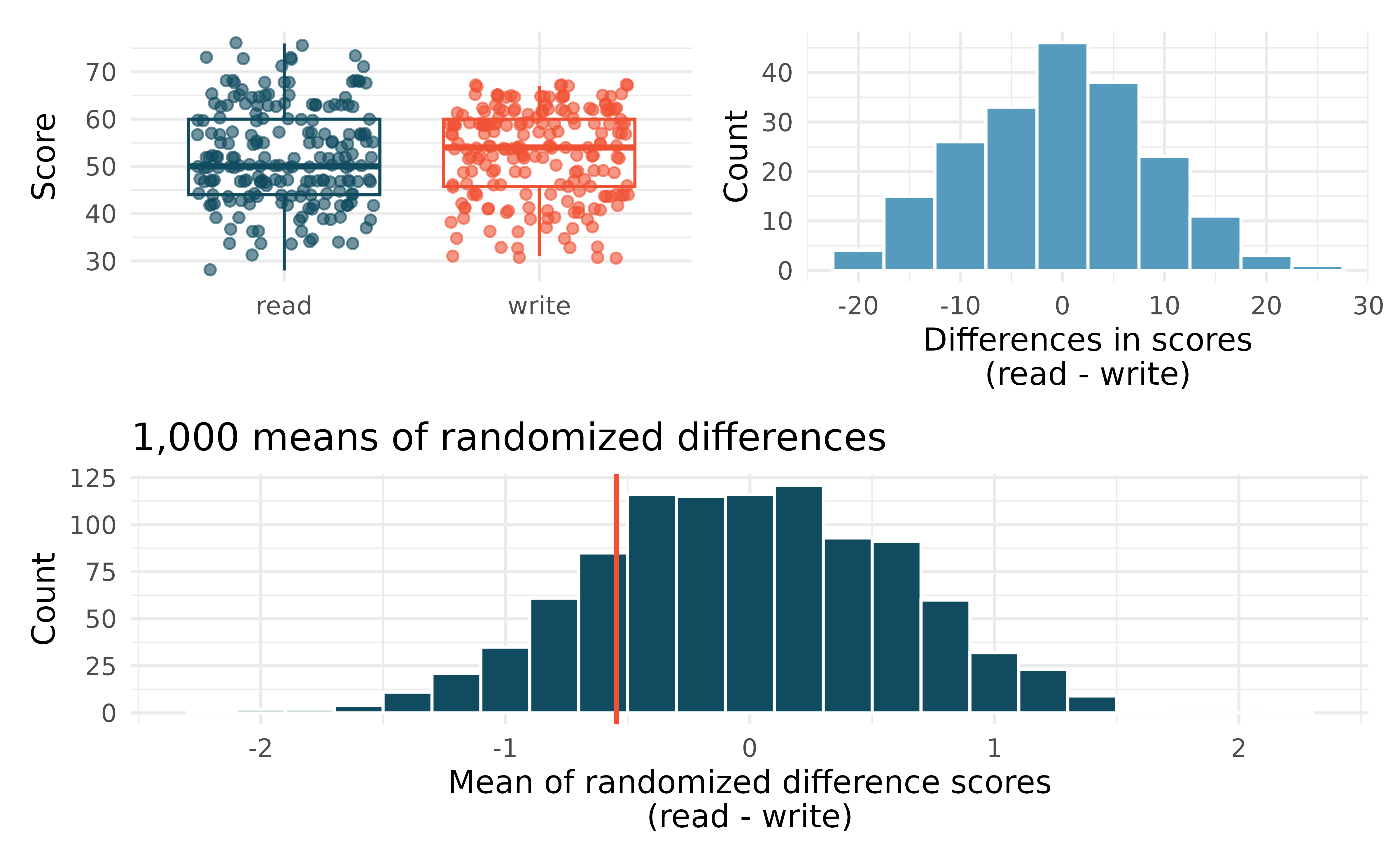
The hsb2 data used in this exercise can be found in the openintro R package.

🔗

Box plots and histograms for High School and Beyond data — Figure 21.34.
🔗

Is there a clear difference in the average reading and writing scores?

🔗
Are the reading and writing scores of each student independent of each other?

🔗
Create hypotheses appropriate for the following research question: is there an evident difference in the average scores of students in the reading and writing exam?

🔗
Is the average of the observed difference in scores $(\bar{x}_{read-write} = -0.545)$ consistent with the distribution of randomized average differences? Explain.

🔗
Do these data provide convincing evidence of a difference between the average scores on the two exams? Estimate the p-value from the randomization test, and conclude the hypothesis test using words like "score on reading test" and "score on writing test."

🔗

🔗

7. Global warming, randomization test.

Let’s consider a limited set of climate data, examining temperature differences in 1950 vs 2022. We sampled 26 locations in the US from the National Oceanic and Atmospheric Administration’s (NOAA) historical data, where the data was available for both years of interest. The data are not a random sample, but they are selected to be a representative sample across the land area of the lower 48 United States. Using the hottest day of the year as a measure can make the results susceptible to outliers. Instead, to get a sense for how hot a year was, we calculate the 90$^{th}$ percentile; that is, we find the maximum temperature on the day that was hotter than 90% of the days that year. We want to know: is the 90$^{th}$ percentile high temperature greater in 2022 or in 1950? The difference in 90$^{th}$ percentile high temperature (high temperature for 2022 - high temperature for 1950) was calculated for each of the 26 locations. The average of the 26 differences was 2.52$^\circ$F with a standard deviation of 2.95$^\circ$F. We are interested in determining whether these data provide strong evidence that the 90$^{th}$ percentile high temperature is higher in 2022 than in 1950.

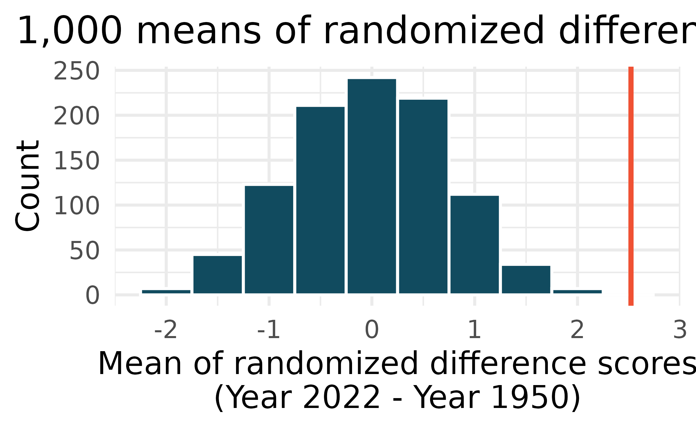
The us_temperature data used in this exercise can be found in the openintro R package.

🔗

Histogram of randomized differences for global warming data — Figure 21.35.
🔗

Create hypotheses appropriate for the following research question: is there an evident difference in the 90$^{th}$ percentile high temp across the two years (1950 and 2022)?

🔗
Is the average of the observed difference in scores $(\bar{x}_{2022-1950} = 2.52^\circ\text{F})$ consistent with the distribution of randomized average differences? Explain.

🔗
Do these data provide convincing evidence of a difference between the 90$^{th}$ percentile high temperature? Estimate the p-value from the randomization test, and conclude the hypothesis test using words like "90$^{th}$ percentile high temperature in 1950" and "90$^{th}$ percentile high temperature in 2022."

🔗

🔗

8. High School and Beyond, bootstrap interval.

We considered the differences between the reading and writing scores of a random sample of 200 students who took the High School and Beyond Survey. The mean and standard deviation of the differences are $\bar{x}_{read-write} = -0.545$ and $s_{read-write} = 8.887$ points. The bootstrap distribution below was produced by bootstrapping from the sample of differences in reading and writing scores 1,000 times.

🔗

Bootstrap distribution for High School and Beyond data — Figure 21.36.
🔗

Find an approximate 95% bootstrap percentile confidence interval for the true average difference in scores (read - write).

🔗
Find an approximate 95% bootstrap SE confidence interval for the true average difference in scores (read - write).

🔗
Interpret both confidence intervals using words like "population" and "score".

🔗
From the confidence intervals calculated above, does it appear that there is a discernible difference in reading and writing scores, on average?

🔗

🔗

9. Global warming, bootstrap interval.

We considered the change in the 90$^{th}$ percentile high temperature in 1950 versus 2022 at 26 sampled locations from the NOAA database. The mean and standard deviation of the reported differences are 2.53$^\circ$F and 2.95$^\circ$F.

🔗

Bootstrap distribution for global warming data — Figure 21.37.
🔗

Calculate a 90% bootstrap percentile confidence interval for the average difference of 90$^{th}$ percentile high temperature between 1950 and 2022.

🔗
Calculate a 90% bootstrap SE confidence interval for the average difference of 90$^{th}$ percentile high temperature between 1950 and 2022.

🔗
Interpret both intervals in context.

🔗
Do the confidence intervals provide convincing evidence that there were hotter high temperatures in 2022 than in 1950 at NOAA stations? Explain your reasoning.

🔗

🔗

10. High School and Beyond, mathematical test.

We considered the differences between the reading and writing scores of a random sample of 200 students who took the High School and Beyond Survey.

🔗

Create hypotheses appropriate for the following research question: is there an evident difference in the average scores of students in the reading and writing exam?

🔗
Check the conditions required to complete this test.

🔗
The average observed difference in scores is $\bar{x}_{read-write} = -0.545\text{,}$ and the standard deviation of the differences is $s_{read-write} = 8.887$ points. Do these data provide convincing evidence of a difference between the average scores on the two exams?

🔗
What type of error might we have made? Explain what the error means in the context of the application.

🔗
Based on the results of this hypothesis test, would you expect a confidence interval for the average difference between the reading and writing scores to include 0? Explain your reasoning.

🔗

🔗

11. Global warming, mathematical test.

🔗

Histogram of differences for global warming data — Figure 21.38.
🔗

Is there a relationship between the observations collected in 1950 and 2022? Or are the observations in the two groups independent? Explain your reasoning.

🔗
Write hypotheses for this research in symbols and in words.

🔗
Check the conditions required to complete this test.

🔗
Calculate the test statistic and find the p-value.

🔗
Use $\alpha = 0.05$ to evaluate the test, and interpret your conclusion in context.

🔗
What type of error might we have made? Explain in context what the error means.

🔗
Based on the results of this hypothesis test, would you expect a confidence interval for the average difference between the 90$^{th}$ percentile high temperature from 1950 to 2022 to include 0? Explain your reasoning.

🔗

🔗

12. High School and Beyond, mathematical interval.

🔗

Calculate a 95% confidence interval for the average difference between the reading and writing scores of all students.

🔗
Interpret this interval in context.

🔗
Does the confidence interval provide convincing evidence that there is a real difference in the average scores? Explain.

🔗

🔗

13. Global warming, mathematical interval.

🔗

Calculate a 90% confidence interval for the average difference of 90$^{th}$ percentile high temperature between 1950 and 2022. We’ve already checked the conditions for you.

🔗
Interpret the interval in context.

🔗
Does the confidence interval provide convincing evidence that there were hotter high temperatures in 2022 than in 1950 at NOAA stations? Explain your reasoning.

🔗

🔗

14. Possible paired randomized differences.

Two observations were collected on each of five people. Which of the following could be a possible randomization of the paired differences given in the table below? If the set of values could not be a randomized set of differences, indicate why not.

🔗

Table 21.39. Paired observations

🔗

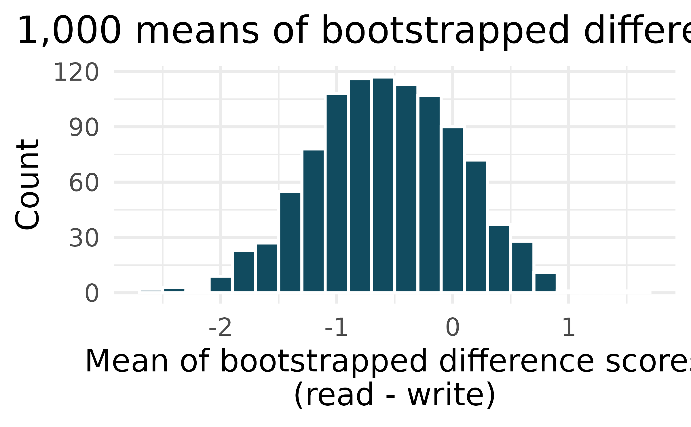
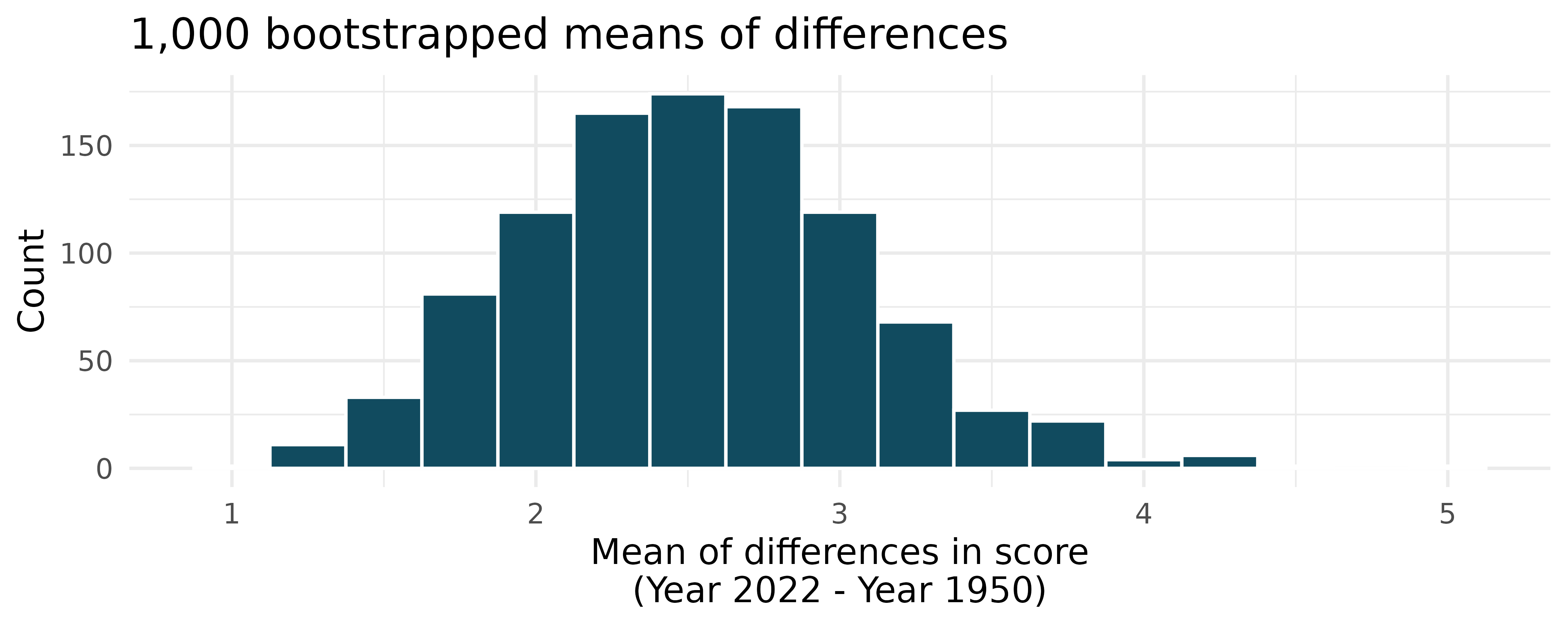
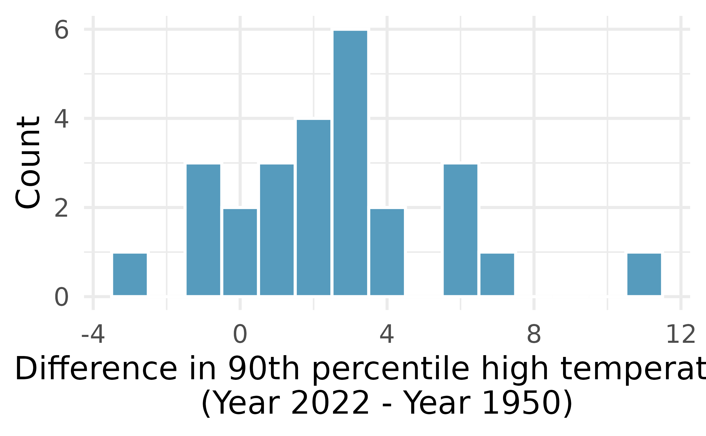
	1	2	3	4	5
Observation 1	3	14	4	5	10
Observation 2	7	3	6	5	9
Difference	-4	11	-2	0	1

-2, 1, 1, 11, -2

🔗
-4, 11, -2, 0, 1

🔗
-2, 2, -11, 11, -2, 2, 0, 1, -1

🔗
0, -1, 2, -4, 11

🔗
4, -11, 2, 0, -1

🔗

🔗

15. Study environment.

In order to test the effects of listening to music while studying versus studying in silence, students agree to be randomized to two treatments (i.e., study with music or study in silence). There are two exams during the semester, so the researchers can either randomize the students to have one exam with music and one with silence (randomly selecting which exam corresponds to which study environment) or the researchers can randomize the students to one study habit for both exams.

🔗

The researchers are interested in estimating the true population difference of exam score for those who listen to music while studying as compared to those who study in silence.

🔗

Describe the experiment which is consistent with a paired designed experiment. How is the treatment assigned, and how are the data collected such that the observations are paired?

🔗
Describe the experiment which is consistent with an independent samples experiment. How is the treatment assigned, and how are the data collected such that the observations are independent?

🔗

🔗

16. Friday the 13th, traffic.

In the early 1990’s, researchers in the UK collected data on traffic flow on Friday the 13th with the goal of addressing issues of how superstitions regarding Friday the 13th affect human behavior and whether Friday the 13th is an unlucky day. The histograms below show the distributions of numbers of cars passing by a specific intersection on Friday the 6th and Friday the 13th for many such date pairs. Also provided are some sample statistics, where the difference is the number of cars on the 6th minus the number of cars on the 13th.

The friday data used in this exercise can be found in the openintro R package.

🔗

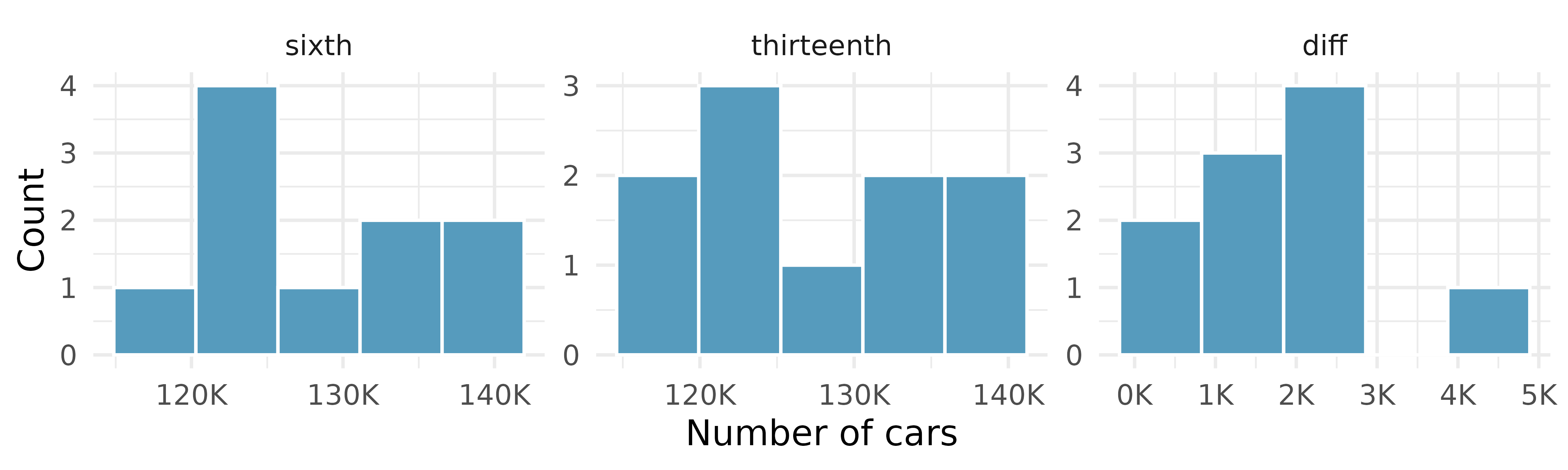
Histograms and summary statistics for Friday the 13th traffic data — Figure 21.40.
🔗

Table 21.41. Summary statistics for Friday the 13th traffic data

🔗

	n	Mean	SD
sixth	10	128,385	7,259
thirteenth	10	126,550	7,664
diff	10	1,836	1,176

Are there any underlying structures in these data that should be considered in an analysis? Explain.

🔗
What are the hypotheses for evaluating whether the number of people out on Friday the 6$^{\text{th}}$ is different than the number out on Friday the 13$^{\text{th}}\text{?}$

🔗
Check conditions to carry out the hypothesis test from part (b) using mathematical models.

🔗
Calculate the test statistic and the p-value.

🔗
What is the conclusion of the hypothesis test?

🔗
Interpret the p-value in this context.

🔗
What type of error might have been made in the conclusion of your test? Explain.

🔗

🔗

17. Friday the 13th, accidents.

In the early 1990’s, researchers in the UK collected data the number of traffic accident related emergency room (ER) admissions on Friday the 13th with the goal of addressing issues of how superstitions regarding Friday the 13th affect human behavior and whether Friday the 13th is an unlucky day. The histograms below show the distributions of numbers of ER admissions at specific emergency rooms on Friday the 6th and Friday the 13th for many such date pairs. Also provided are some sample statistics, where the difference is the ER admissions on the 6th minus the ER admissions on the 13th.

⁴

The friday data used in this exercise can be found in the openintro R package.

🔗

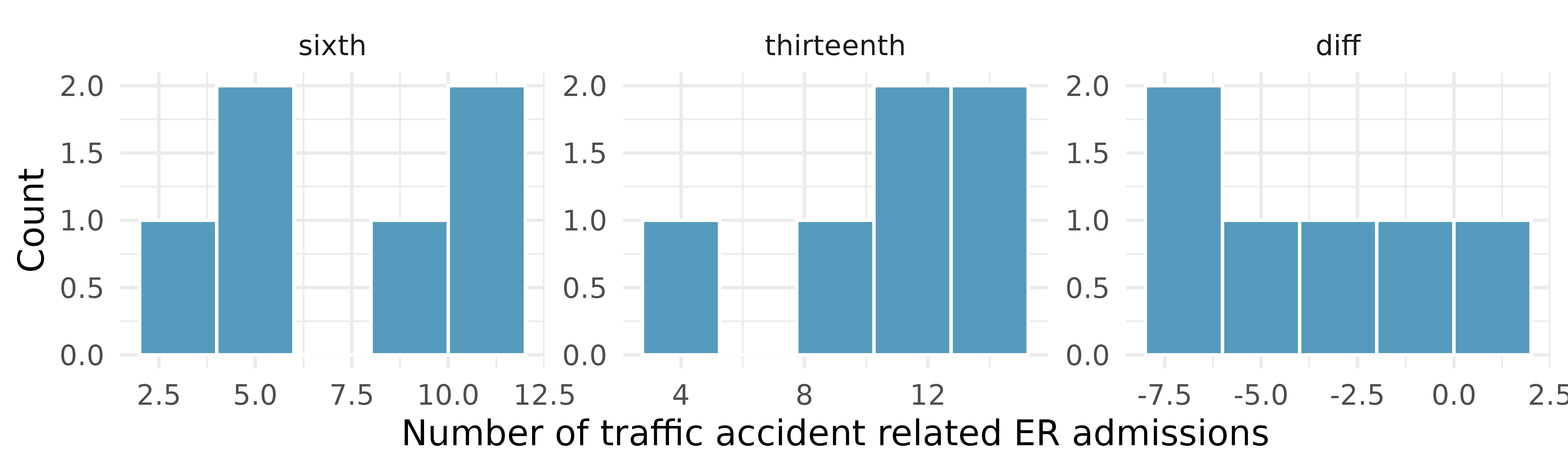
Histograms and summary statistics for Friday the 13th accidents data — Figure 21.42.
🔗

Table 21.43. Summary statistics for Friday the 13th accidents data

🔗

	n	Mean	SD
sixth	6	8	3
thirteenth	6	11	4
diff	6	-3	3

Conduct a hypothesis test using mathematical models to evaluate if there is a difference between the average numbers of traffic accident related emergency room admissions between Friday the 6$^{\text{th}}$ and Friday the 13$^{\text{th}}\text{.}$

🔗
Calculate a 95% confidence interval using mathematical models for the difference between the average numbers of traffic accident related emergency room admissions between Friday the 6$^{\text{th}}$ and Friday the 13$^{\text{th}}\text{.}$

🔗
The conclusion of the original study states, "Friday 13th is unlucky for some. The risk of hospital admission as a result of a transport accident may be increased by as much as 52%. Staying at home is recommended." Do you agree with this statement? Explain your reasoning.

🔗

🔗

18. Forest management.

Forest rangers wanted to better understand the rate of growth for younger trees in the park. They took measurements of a random sample of 50 young trees in 2009 and again measured those same trees in 2019. The data below summarize their measurements, where the heights are in feet.

🔗

Table 21.44. Tree growth data

🔗

Year	Mean	SD	n
2009	12	3.5	50
2019	24.5	9.5	50
Difference	12.5	7.2	50

Construct a 99% confidence interval for the average growth of (what had been) younger trees in the park over 2009-2019.

🔗

Prev Top Next