In Chapter 17 our focus was on the difference in proportions, a statistic calculated from finding the success proportions (from the binary response variable) measured across two groups (the binary explanatory variable). As we will see in the examples below, sometimes the explanatory or response variables have more than two possible options. In that setting, a difference across two groups is not sufficient, and the proportion of “success” is not well defined if there are 3 or 4 or more possible response levels. The primary way to summarize categorical data where the explanatory and response variables both have 2 or more levels is through a two-way table as in Table 18.1.
Note that with two-way tables, there is not an obvious single parameter of interest. Instead, research questions usually focus on how the proportions of the response variable changes (or not) across the different levels of the explanatory variable. Because there is not a population parameter to estimate, bootstrapping to find the standard error of the estimate is not meaningful. As such, for two-way tables, we will focus on the randomization test and corresponding mathematical approximation (and not bootstrapping).
We all buy used products — cars, computers, textbooks, and so on — and we sometimes assume the sellers of those products will be forthright about any underlying problems with what they’re selling. This is not something we should take for granted. Researchers recruited 219 participants in a study where they would sell a used iPod 1
iPod
that was known to have frozen twice in the past. The participants were incentivized to get as much money as they could for the iPod since they would receive a 5% cut of the sale on top of $10 for participating. The researchers wanted to understand what types of questions would elicit the seller to disclose the freezing issue.
Unbeknownst to the participants who were the sellers in the study, the buyers were collaborating with the researchers to evaluate the influence of different questions on the likelihood of getting the sellers to disclose the past issues with the iPod. The scripted buyers started with “Okay, I guess I’m supposed to go first. So you’ve had the iPod for 2 years ...” and ended with one of three questions:
The question is the treatment given to the sellers, and the response is whether the question prompted them to disclose the freezing issue with the iPod. The results are shown in Table 18.1, and the data suggest that asking the, What problems does it have?, was the most effective at getting the seller to disclose the past freezing issues. However, you should also be asking yourself: could we see these results due to chance alone if there really is no difference in the question asked, or is this in fact evidence that some questions are more effective for getting at the truth?
See the table showing summary of the iPod study, where a question was posed to the study participant who acted (with columns for Question, Disclose problem, Hide problem, and Total).
The hypothesis test for the iPod experiment is really about assessing whether there is convincing evidence that there was a difference in the success rates that each question had on getting the participant to disclose the problem with the iPod. In other words, the goal is to check whether the buyer’s question was independent of whether the seller disclosed a problem.
While we would not expect the number of disclosures to be exactly the same across the three question classes, the rate of disclosure seems substantially different across the three groups. In order to investigate whether the differences in rates is due to natural variability in people’s honesty or due to a treatment effect (i.e., the question causing the differences), we need to compute estimated counts for each cell in a two-way table.
From the experiment, we can compute the proportion of all sellers who disclosed the freezing problem as \(61/219 = 0.2785.\) If there really is no difference among the questions and 27.85% of sellers were going to disclose the freezing problem no matter the question they were asked, how many of the 73 people in the General group would we have expected to disclose the freezing problem?
We would predict that \(0.2785 \times 73 = 20.33\) sellers would disclose the problem. Obviously we observed fewer than this, though it is not yet clear if that is due to chance variation or whether that is because the questions vary in how effective they are at getting to the truth.
If the questions were actually equally effective, meaning about 27.85% of respondents would disclose the freezing issue regardless of what question they were asked, about how many sellers would we expect to hide the freezing problem from the Positive Assumption group?
We can compute the expected number of sellers who we would expect to disclose or hide the freezing issue for all groups, if the questions had no impact on what they disclosed, using the same strategies employed in the previous Example and Guided Practice to compute expected counts. These expected counts were used to construct Table 18.4, which is the same as Table 18.1, except now the expected counts have been added in parentheses.
The examples and exercises above provided some help in computing expected counts. In general, expected counts for a two-way table may be computed using the row totals, column totals, and the table total. For instance, if there was no difference between the groups, then about 27.85% of each row should be in the first column:
Looking back to how 0.2785 was computed — as the fraction of sellers who disclosed the freezing issue \((61/219)\) — these three expected counts could have been computed as
This leads us to a general formula for computing expected counts in a two-way table when we would like to test whether there is strong evidence of an association between the column variable and row variable.
The chi-squared test statistic for a two-way table is found by finding the ratio of how far the observed counts are from the expected counts, as compared to the expected counts, for every cell in the table. For each table count, compute:
Is 40.13 a big number? That is, does it indicate that the observed and expected values are really different? Or is 40.13 a value of the statistic that we would expect to see just due to natural variability? Previously, we applied the randomization test to the setting where the research question investigated a difference in proportions. The same idea of shuffling the data under the null hypothesis can be used in the setting of the two-way table.
Assuming that the individuals would disclose or hide the problems regardless of the question they are given (i.e., that the null hypothesis is true), we can randomize the data by reassigning the 61 disclosed problems and 158 hidden problems to the three groups at random. Table 18.5 shows a possible randomization of the observed data under the condition that the null hypothesis is true (in contrast to the original observed data in Table 18.1).
As before, the randomized data is used to find a single value for the test statistic (here a chi-squared statistic). The chi-squared statistic for the randomized two-way table is found by comparing the observed and expected counts for each cell in the randomized table. For each cell, compute:
Subsection18.1.4Observed statistic vs. null chi-squared statistics
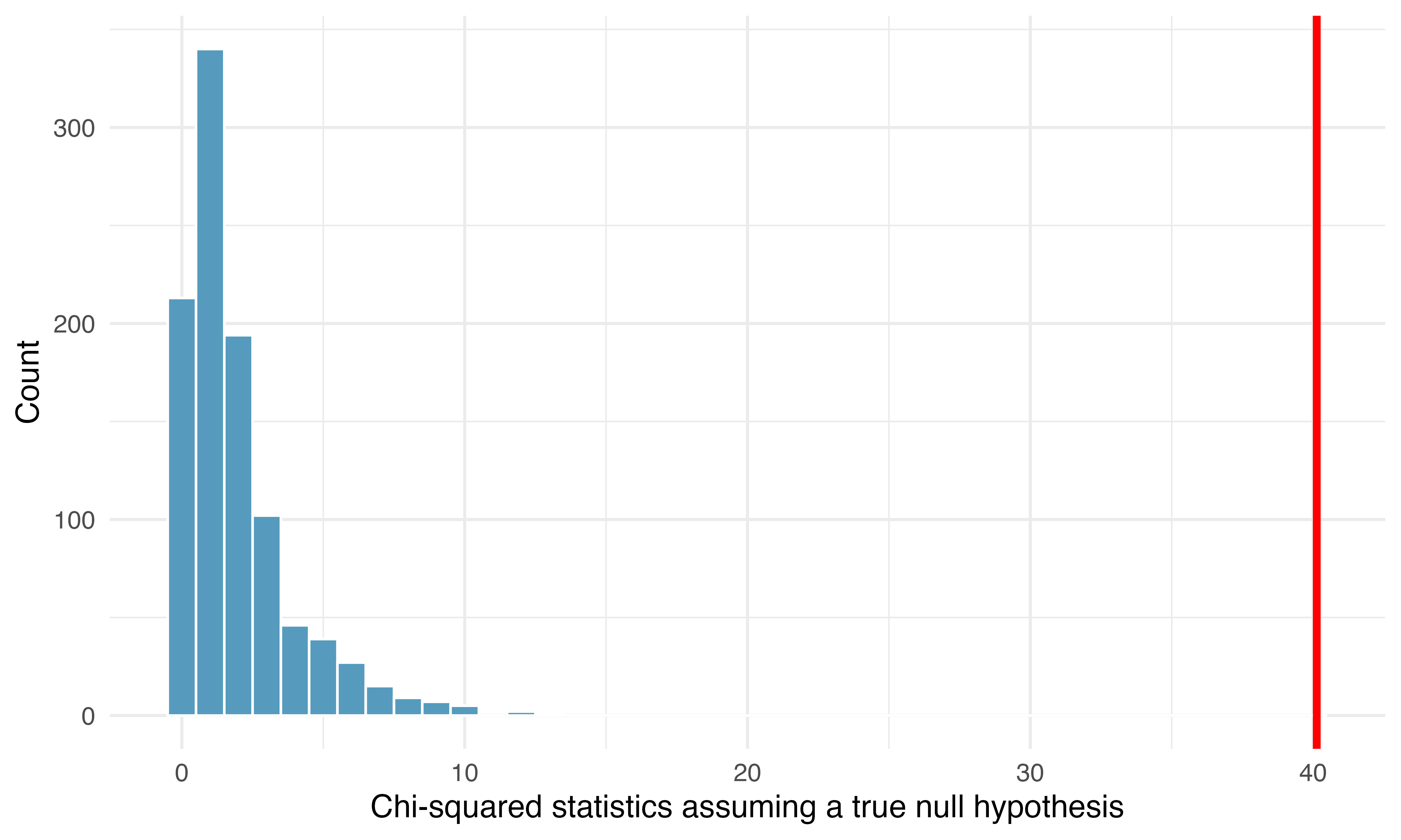
As before, one randomization will not be sufficient for understanding if the observed data are particularly different from the expected chi-squared statistics when \(H_0\) is true. To investigate whether 40.13 is large enough to indicate the observed and expected counts are substantially different, we need to understand the variability in the values of the chi-squared statistic we would expect to see if the null hypothesis was true. Figure 18.6 plots 1,000 chi-squared statistics generated under the null hypothesis. We can see that the observed value is so far from the null statistics that the simulated p-value is zero. That is, the probability of seeing the observed statistic when the null hypothesis is true is virtually zero. In this case we can conclude that the decision of whether to disclose the iPod’s problem is changed by the question asked. We use the causal language of “changed” because the study was an experiment. Note that with a chi-squared test, we only know that the two variables (question_class and response) are related (i.e., not independent). We are not able to claim which type of question causes which type of response.
Figure18.6.A histogram of chi-squared statistics from 1,000 simulations produced under the null hypothesis, \(H_0,\) where the question is independent of the response. The observed statistic of 40.13 is marked by the red line. None of the 1,000 simulations had a chi-squared value of at least 40.13. In fact, none of the simulated chi-squared statistics came anywhere close to the observed statistic!
Section18.2Mathematical model for test of independence
Subsection18.2.1The chi-squared test of independence
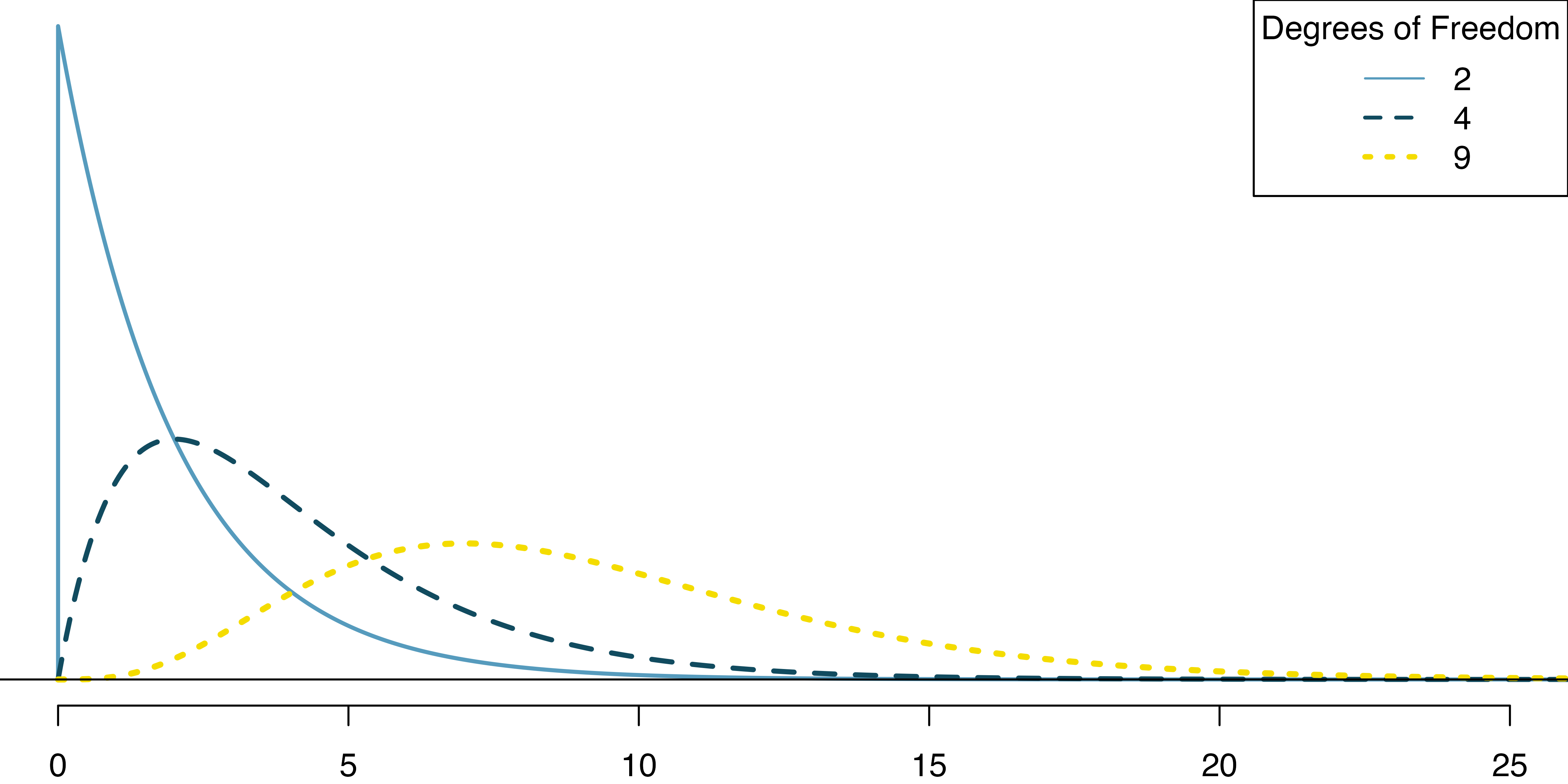
Previously, in Section 17.3, we applied the Central Limit Theorem to the sampling variability of \(\hat{p}_1 - \hat{p}_2.\) The result was that we could use the normal distribution (e.g., \(z^*\) values (see Figure 16.11) and p-values from \(Z\) scores) to complete the mathematical inferential procedure. The chi-squared test statistic has a different mathematical distribution called the Chi-squared distribution. The important specification to make in describing the chi-squared distribution is something called degrees of freedom. The degrees of freedom change the shape of the chi-squared distribution to fit the problem at hand. Figure 18.7 visualizes different chi-squared distributions corresponding to different degrees of freedom.
Figure18.7.The chi-squared distribution for differing degrees of freedom. The larger the degrees of freedom, the longer the right tail extends. The smaller the degrees of freedom, the more peaked the mode on the left becomes.
Subsection18.2.2Variability of the chi-squared statistic
As it turns out, the chi-squared test statistic follows a Chi-squared distribution when the null hypothesis is true. For two way tables, the degrees of freedom is equal to: \(df = \text{(number of rows minus 1)}\times \text{(number of columns minus 1)}\text{.}\) In our example, the degrees of freedom parameter is \(df = (2-1)\times (3-1) = 2\text{.}\)
Subsection18.2.3Observed statistic vs. null chi-squared statistics
The test statistic for assessing the independence between two categorical variables is a \(X^2\).
The \(X^2\) statistic is a ratio of how the observed counts vary from the expected counts as compared to the expected counts (which are a measure of how large the sample size is).
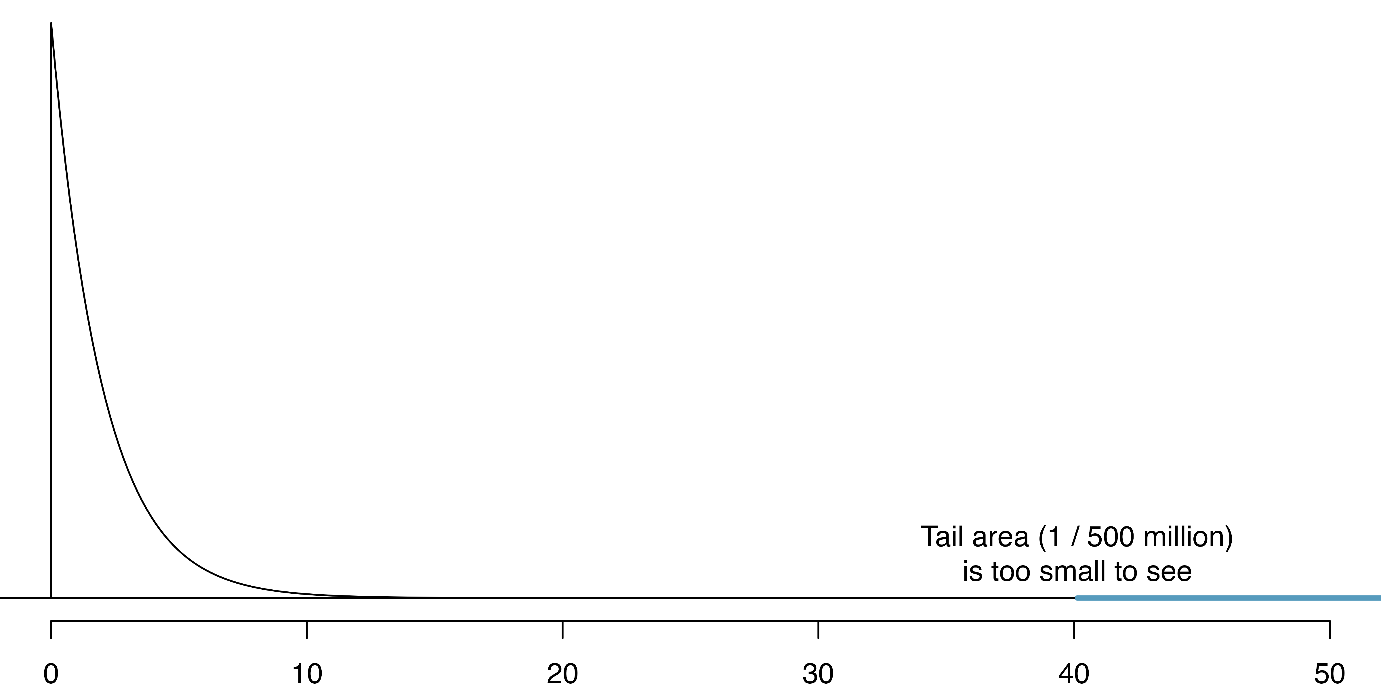
To bring it back to the example, we can safely assume that the observations are independent, as the question groups were randomly assigned. Additionally, there are over 5 expected counts in each cell, so the conditions for using the Chi-square distribution are met. If the null hypothesis is true (i.e., the questions had no impact on the sellers in the experiment), then the test statistic \(X^2 = 40.13\) is expected to follow a Chi-squared distribution with 2 degrees of freedom. Using this information, we can compute the p-value for the test, which is depicted in Figure 18.8.
When applying the chi-squared test to a two-way table, we use \(df = (R-1)\times (C-1)\) where \(R\) is the number of rows in the table and \(C\) is the number of columns.
The software R can be used to find the p-value with the function pchisq(). Just like pnorm(), pchisq() always gives the area to the left of the cutoff value. Because, in this example, the p-value is represented by the area to the right of 40.13, we subtract the output of pchisq() from 1.
Using a computer, we can compute a very precise value for the tail area above \(X^2 = 40.13\) for a chi-squared distribution with 2 degrees of freedom: 0.000000002.
Using a discernibility level of \(\alpha=0.05,\) the null hypothesis is rejected since the p-value is smaller. That is, the data provide convincing evidence that the question asked did affect a seller’s likelihood to tell the truth about problems with the iPod.
See the table showing results for the Type 2 Diabetes study (with columns for Treatment, Failure, Success, and Total). The table summarizes the results of an experiment evaluating three treatments for Type 2 Diabetes in patients aged 10-17 who were being treated with metformin. The three treatments considered were continued treatment with metformin (met), treatment with metformin combined with rosiglitazone (rosi), or a lifestyle intervention program. Each patient had a primary outcome, which was either lacked glycemic control (failure) or did not lack that control (success). What are appropriate hypotheses for this test?
Typically we will use a computer to do the computational work of finding the chi-squared statistic. However, it is always good to have a sense for what the computer is doing, and in particular, calculating the values which would be expected if the null hypothesis is true can help to understand the null hypothesis claim. Additionally, comparing the expected and observed values by eye often gives the researcher some insight into why or why not the null hypothesis for a given test is rejected or not.
A chi-squared test for a two-way table may be used to test the hypotheses in the diabetes Example above. To get a sense for the statistic used in the chi-squared test, first compute the expected values for each of the six table cells.
The expected count for row one / column one is found by multiplying the row one total (234) and column one total (319), then dividing by the table total (699): \(\frac{234\times 319}{699} = 106.8.\) Similarly for the second column and the first row: \(\frac{234\times 380}{699} = 127.2.\) Row 2: 105.9 and 126.1. Row 3: 106.3 and 126.7.
Note, when analyzing 2-by-2 contingency tables (that is, when both variables only have two possible options), one guideline is to use the two-proportion methods introduced in Chapter 17.
In this chapter we extended the randomization / bootstrap / mathematical model paradigm to research questions involving categorical variables. We continued working with one population proportion as well as the difference in populations proportions, but the test of independence allowed for hypothesis testing on categorical variables with more than two levels. We note that the normal model was an excellent mathematical approximation to the sampling distribution of sample proportions (or differences in sample proportions), but that the questions with categorical variables with more than 2 levels required a new mathematical model, the chi-squared distribution. As seen in Chapter 11, Chapter 12 and Chapter 13, almost all the research questions can be approached using computational methods (e.g., randomization tests or bootstrapping) or using mathematical models. We continue to emphasize the importance of experimental design in making conclusions about research claims. In particular, recall that variability can come from different sources (e.g., random sampling vs. random allocation, see Figure 2.16).
The terms introduced in this chapter are presented in Table 18.13. If you’re not sure what some of these terms mean, we recommend you go back in the text and review their definitions. You should be able to easily spot them as bolded text.
Does being part of a support group affect the ability of people to quit smoking? A county health department enrolled 300 smokers in a randomized experiment. 150 participants were randomly assigned to a group that used a nicotine patch and met weekly with a support group; the other 150 received the patch and did not meet with a support group. At the end of the study, 40 of the participants in the patch plus support group had quit smoking while only 30 smokers had quit in the other group.
Answer each of the following questions under the null hypothesis that being part of a support group does not affect the ability of people to quit smoking, and indicate whether the expected values are higher or lower than the observed values.
The table below summarizes results from a Pew Research poll which asked respondents whether they have personally taken action to help address climate change within the last year and their generation. The differences in each generational group may be due to chance. Complete the following computations under the null hypothesis of independence between an individual’s generation and whether they have personally taken action to help address climate change within the last year. [47]
In order to assess whether habitat conditions are related to the sunlight choices a lizard makes for resting, Western fence lizard (Sceloporus occidentalis) were observed across three different microhabitats. [48][49]
If the variables describing the habitat and the amount of sunlight are independent, what proportion of lizards (total) would be expected in each of the three sunlight categories?
Compare the observed (original data) and expected (part b.) tables. From a first glance, does it seem as though the habitat and choice of sunlight may be associated?
Regardless of your answer to part (c), is it possible to tell from looking only at the expected and observed counts whether the two variables are associated?
4.Disaggregating Asian American tobacco use, data.
Understanding cultural differences in tobacco use across different demographic groups can lead to improved health care education and treatment. A recent study disaggregated tobacco use across Asian American ethnic groups including Asian-Indian (n = 4,373), Chinese (n = 4,736), and Filipino (n = 4,912), in comparison to non-Hispanic Whites (n = 275,025). The number of current smokers in each group was reported as Asian-Indian (n = 223), Chinese (n = 279), Filipino (n = 609), and non-Hispanic Whites (n = 50,880). [50]
In order to assess whether there is a difference in current smoking rates across three Asian American ethnic groups, the observed data is compared to the data that would be expected if there were no association between the variables.
Compare the observed and expected counts. From a first glance, does it seem as though the Asian American ethnicity and choice of smoking may be associated?
Regardless of your answer to part (c), is it possible to tell from looking only at the expected and observed counts whether the two variables are associated?
In order to assess whether habitat conditions are related to the sunlight choices a lizard makes for resting, Western fence lizard (Sceloporus occidentalis) were observed across three different microhabitats. [48][49] Then, the data were randomized once, where sunlight preference was randomly assigned to the lizards across different sites. The original data are shown on the left and the results of the randomization is shown on the right.
Recall that the Chi-squared statistic \((X^2)\) measures the difference between the expected and observed counts. Without calculating the actual statistic, report on whether the original data or the randomized data will have a larger Chi-squared statistic. Explain your choice.
6.Disaggregating Asian American tobacco use, randomize once.
In a study that aims to disaggregate tobacco use across Asian American ethnic groups (Asian-Indian, Chinese, and Filipino, in comparison to non-Hispanic Whites), respondents were asked whether they smoke tobacco or not. [50] Then, the data were randomized once, where smoking status was randomly assigned to the participants across different ethnicities. The original data are shown on the left and the results of the randomization is shown on the right.
Recall that the Chi-squared statistic \((X^2)\) measures the difference between the expected and observed counts. Without calculating the actual statistic, report on whether the original data or the randomized data will have a larger Chi-squared statistic. Explain your choice.
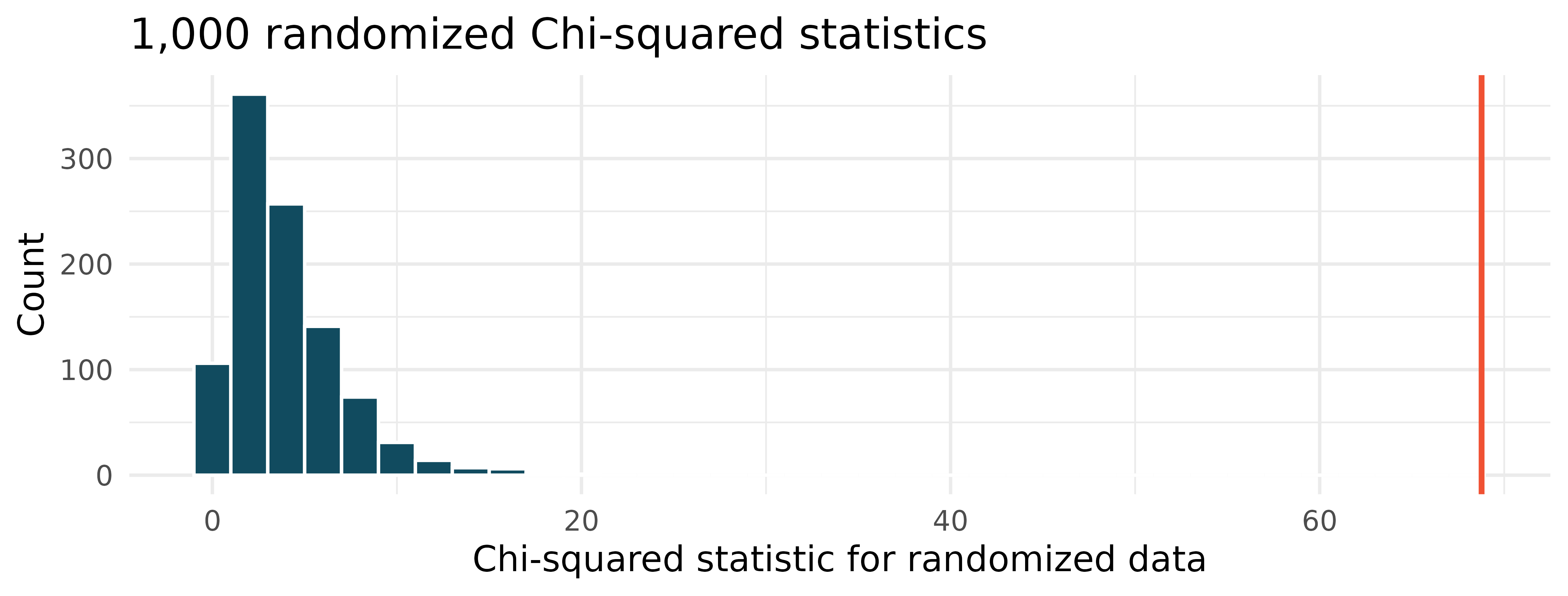
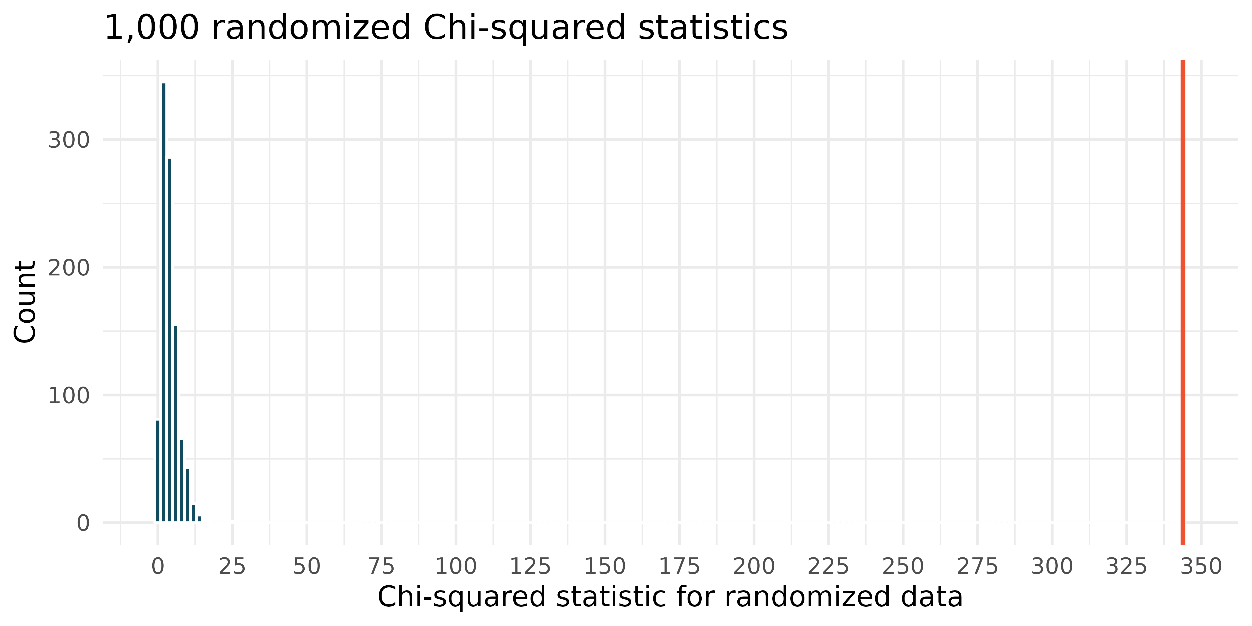
In order to assess whether habitat conditions are related to the sunlight choices a lizard makes for resting, Western fence lizard (Sceloporus occidentalis) were observed across three different microhabitats. [48][49] The original data were randomized 1,000 times (sunlight variable randomly assigned to the observations across different habitats), and the histogram of the Chi-squared statistic on each randomization is displayed.
The histogram above describes the Chi-squared statistics for 1,000 different randomization datasets. When randomizing the data, is the imposed structure that the variables are independent or that the variables are associated? Explain.
The observed Chi-squared statistic is 68.8 (marked in red on plot). Does the observed value provide evidence against the null hypothesis? To answer the question, state the null and alternative hypotheses, approximate the p-value, and conclude the test in the context of the problem.
8.Disaggregating Asian American tobacco use, randomization test.
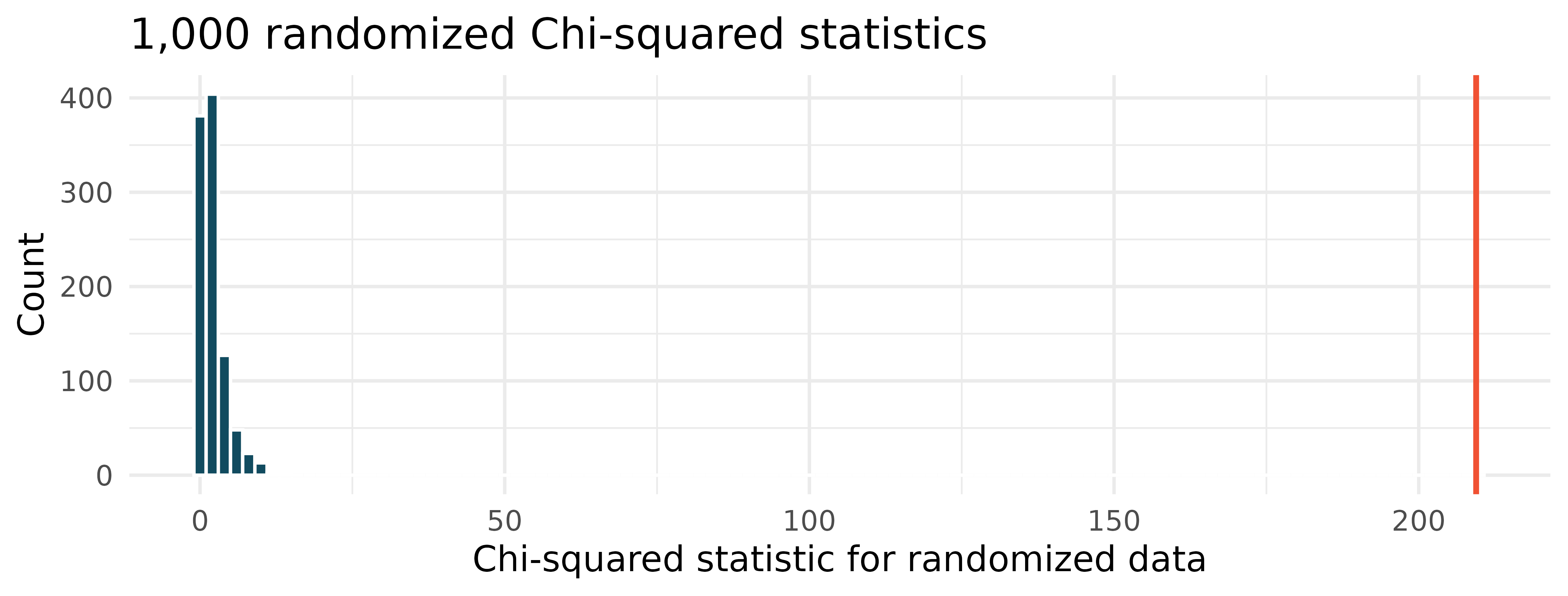
Understanding cultural differences in tobacco use across different demographic groups can lead to improved health care education and treatment. A recent study disaggregated tobacco use across Asian American ethnic groups including Asian-Indian (n = 4373), Chinese (n = 4736), and Filipino (n = 4912), in comparison to non-Hispanic Whites (n = 275,025). The number of current smokers in each group was reported as Asian-Indian (n = 223), Chinese (n = 279), Filipino (n = 609), and non-Hispanic Whites (n = 50,880). [50] The original data were randomized 1000 times (smoking status randomly assigned to the observations across ethnicities), and the histogram of the Chi-squared statistic on each randomization is displayed.
The histogram above describes the Chi-squared statistics for 1000 different randomization datasets. When randomizing the data, is the imposed structure that the variables are independent or that the variables are associated? Explain.
The observed Chi-squared statistic is 209.42 (marked in red on plot). Does the observed value provide evidence against the null hypothesis? To answer the question, state the null and alternative hypotheses, approximate the p-value, and conclude the test in the context of the problem.
In order to assess whether habitat conditions are related to the sunlight choices a lizard makes for resting, Western fence lizard (Sceloporus occidentalis) were observed across three different microhabitats. [48][49]
Consider the situation where the dataset is 5 times larger than the original data (but have the same proportional representation in each category). The distribution of lizards in each of the sites resting in the sun, partial sun, and shade are as follows.
The larger dataset was randomized 1,000 times (sunlight preference randomly assigned to the observations across sites), and the histogram of the Chi-squared statistic on each randomization is displayed.
The histogram above describes the Chi-squared statistics for 1,000 different randomization of the larger dataset. When randomizing the data, is the imposed structure that the variables are independent or that the variables are associated? Explain.
The observed Chi-squared statistic is \(X^2_{\text{obs}}\) (and seen in red on the graph). Does the observed value provide evidence against the null hypothesis? To answer the question, state the null and alternative hypotheses, approximate the p-value, and conclude the test in the context of the problem.
If the alternative hypothesis is true, how does the sample size effect the ability to reject the null hypothesis? (Hint: Consider the original data as compared with the larger dataset that have the same proportional values.)
10.Disaggregating Asian American tobacco use, smaller data.
Understanding cultural differences in tobacco use across different demographic groups can lead to improved health care education and treatment. A recent study disaggregated tobacco use across Asian American ethnic groups. [50]
Consider the situation where the dataset is 50 times smaller than the original data (but have the same proportional representation in each category). The distribution of smokers in each of the ethnicity groups in the smaller data are as follows.
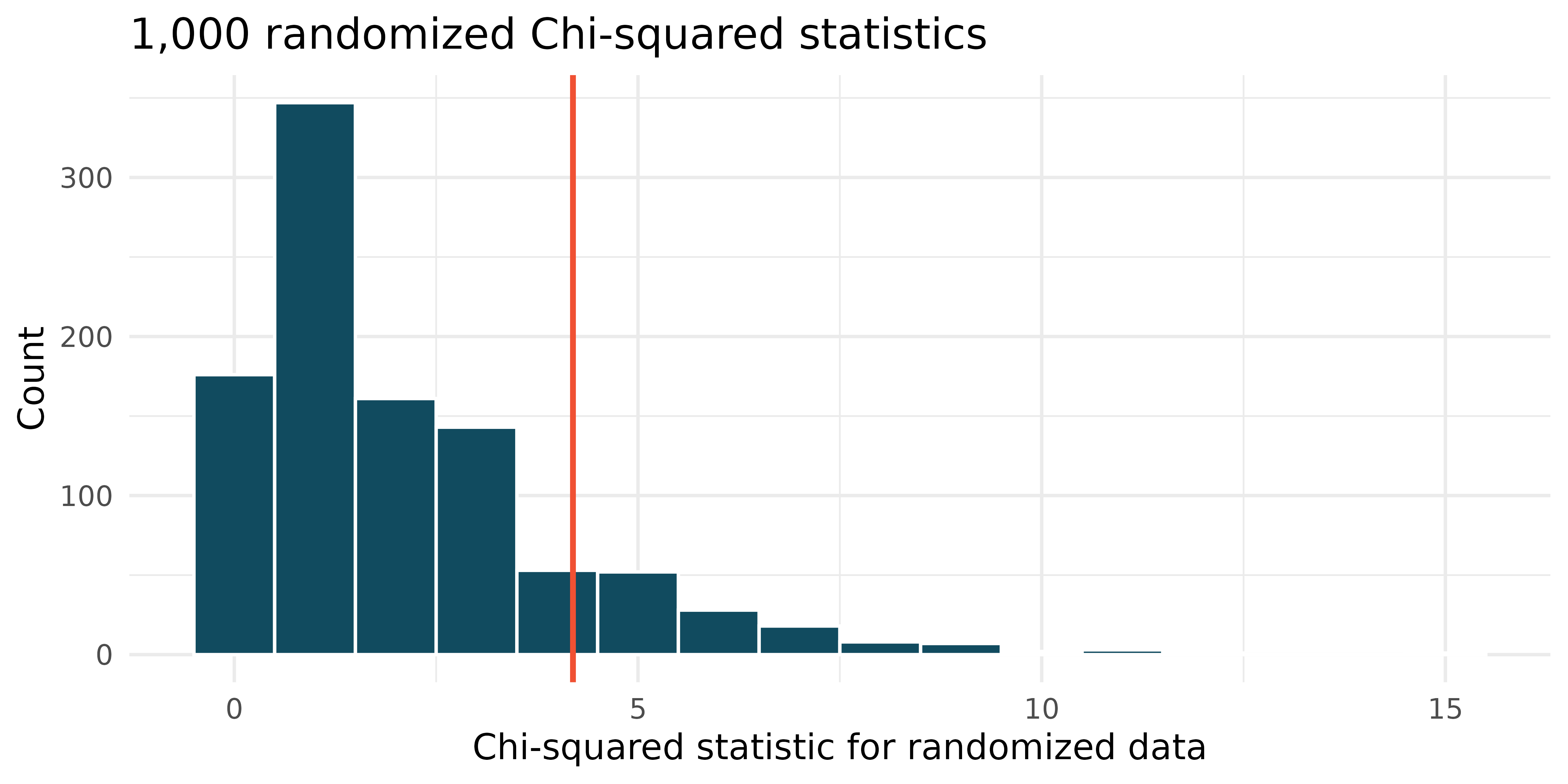
The smaller dataset was randomized 1,000 times (smoking status randomly assigned to the observations across ethnicities), and the histogram of the Chi-squared statistic on each randomization is displayed.
The histogram above describes the Chi-squared statistics for 1,000 different randomization of the smaller dataset. When randomizing the data, is the imposed structure that the variables are independent or that the variables are associated? Explain.
The observed Chi-squared statistic is 4.19 (and seen in red on the graph). Does the observed value provide evidence against the null hypothesis? To answer the question, state the null and alternative hypotheses, approximate the p-value, and conclude the test in the context of the problem.
If the alternative hypothesis is true, how does the sample size effect the ability to reject the null hypothesis? (Hint: Consider the original data as compared with the smaller dataset that have the same proportional values.)
The National Sleep Foundation conducted a survey on the sleep habits of randomly sampled transportation workers and randomly sampled non-transportation workers that serve as a "control" for comparison. [51] The results of the survey are shown below. Conduct a hypothesis test to evaluate if these data provide evidence of an association between sleep levels and profession.
Lymphatic filariasis is a disease caused by a parasitic worm. Complications of the disease can lead to extreme swelling and other complications. Here we consider results from a randomized experiment that compared three different drug treatment options to clear people of the this parasite, which people are working to eliminate entirely. The results for the second year of the study are given below: [60]
Statistical software was used to run a Chi-square test, which output: \(X^2 = 23.7 \quad df = 2 \quad \text{p-value} < 0.0001\text{.}\) Use these results to evaluate the hypotheses from part (a), and provide a conclusion in the context of the problem.
A local news survey asked 500 randomly sampled Los Angeles residents which shipping carrier they prefer to use for shipping holiday gifts. The table below shows the distribution of responses by age group as well as the expected counts for each cell (shown in brackets).
State the null and alternative hypotheses for testing for independence of age and preferred shipping method for holiday gifts among Los Angeles residents.
Researchers conducted a study investigating the relationship between caffeinated coffee consumption and risk of depression in women. They collected data on 50,739 women free of depression symptoms at the start of the study in the year 1996, and these women were followed through 2006. The researchers used questionnaires to collect data on caffeinated coffee consumption, asked each individual about physician- diagnosed depression, and also asked about the use of antidepressants. The table below shows the distribution of incidences of depression by amount of caffeinated coffee consumption. [59]
One of the authors of this study was quoted on the New York Times as saying it was "too early to recommend that women load up on extra coffee" based on just this study. [40] Do you agree with this statement? Explain your reasoning.