Chapter25Inference for linear regression with multiple predictors
In Chapter 8, the least squares regression method was used to estimate linear models which predicted a particular response variable given more than one explanatory variable.
Here, we discuss whether each of the variables individually is a statistically discernible predictor of the outcome or whether the model might be just as strong without that variable.
That is, as before, we apply inferential methods to ask whether a variable could have come from a population where the particular coefficient at hand was zero.
If one of the linear model coefficients is truly zero (in the population), then the estimate of the coefficient (using least squares) will vary around zero.
The inference task at hand is to decide whether the coefficient’s difference from zero is large enough to decide that the data cannot possibly have come from a model where the true population coefficient is zero.
Both the derivations from the mathematical model and the randomization model are beyond the scope of this book, but we are able to calculate p-values using statistical software.
We will discuss interpreting p-values in the multiple regression setting and note some scenarios where careful understanding of the context and the relationship between variables is important.
Based on the data in this dataset we have created two new variables: credit_util which is calculated as the total credit utilized divided by the total credit limit and bankruptcy which turns the number of bankruptcies to an indicator variable (0 for no bankruptcies and 1 for at least 1 bankruptcy).
Table25.3.Summary of a linear model for predicting interest rate based on debt_to_income, term, and credit_checks. Each of the variables has its own coefficient estimate as well as a p-value.
Not only does Table 25.3 provide the estimates for the coefficients, it also provides information on the inference analysis (i.e., hypothesis testing) which is the focus of this chapter.
In Chapter 24, you learned that the hypothesis test for a linear model with one predictor 1
In previous sections, the term explanatory variable was used instead of predictor. The words are synonymous and are used separately in the different sections to be consistent with how most analysts use them: explanatory variable for testing, predictor for modeling.
That is, if the true population slope is zero, the p-value measures how likely it would be to select data which produced the observed slope \((b_1)\) value.
Using the example above and focusing on each of the variable p-values (here we won’t discuss the p-value associated with the intercept), we can write out the three different hypotheses:
The very low p-values from the software output tell us that each of the variables acts as an important predictor in the model, despite the inclusion of the other two. Consider the p-value on \(H_0: \beta_1 = 0\text{.}\) The low p-value says that it would be extremely unlikely to see data that produce a coefficient on debt_to_income as large as 0.041 if the true relationship between debt_to_income and interest_rate was non-existent (i.e., if \(\beta_1 = 0\)) and the model also included term and credit_checks. You might have thought that the value 0.041 is a small number (i.e., close to zero), but in the units of the problem, 0.041 turns out to be far away from zero, it’s all about context! The p-values on term and on credit_checks are interpreted similarly.
In practice, there will almost always be some degree of correlation between the explanatory variables in a multiple regression model. For regression models, it is important to understand the entire context of the model, particularly for correlated variables. Our discussion will focus on interpreting coefficients (and their signs) in relationship to other variables as well as the discernibility (i.e., the p-value) of each coefficient.
Consider an example where we would like to predict how much money is in a coin dish based only on the number of coins in the dish. We ask 26 students to tell us about their individual coin dishes, collecting data on the total dollar amount, the total number of coins, and the total number of low coins. 2
In all honesty, this particular dataset is fabricated, and the original idea for the problem comes from Jeff Witmer at Oberlin College.
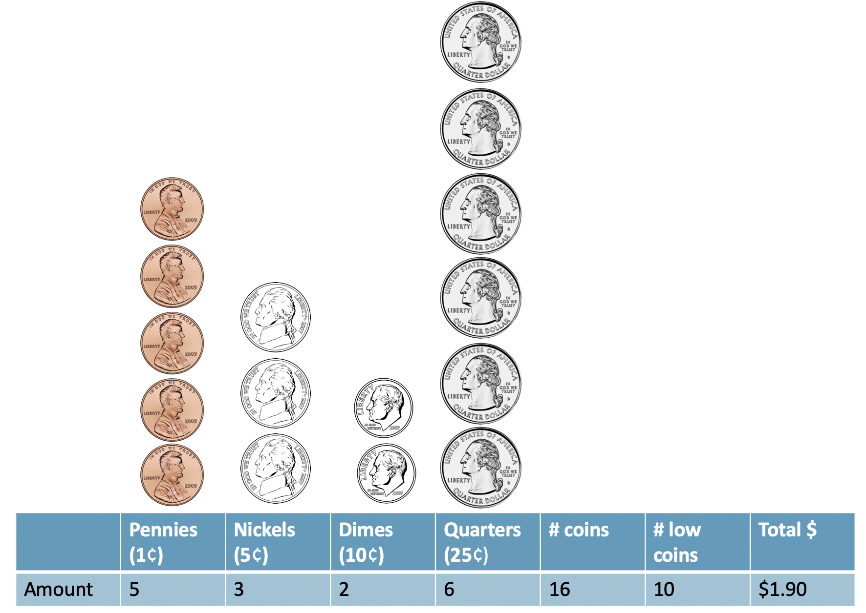
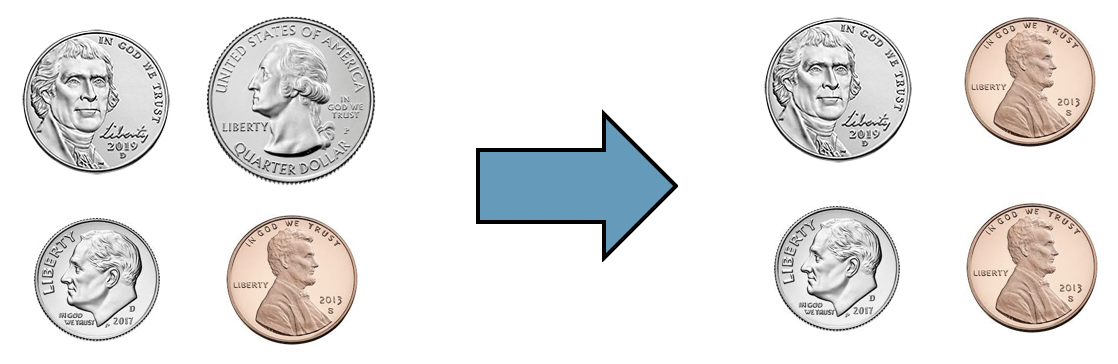
The number of low coins is the number of coins minus the number of quarters (a quarter is the largest commonly used US coin, at US$0.25). Figure 25.4 illustrates a sample of U.S. coins, their total worth (total_amount), the total number_of_coins, and the number_of_low_coins.
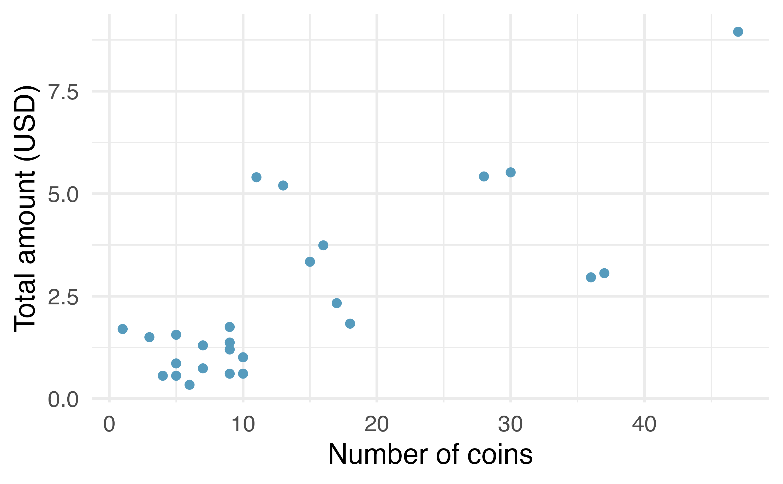
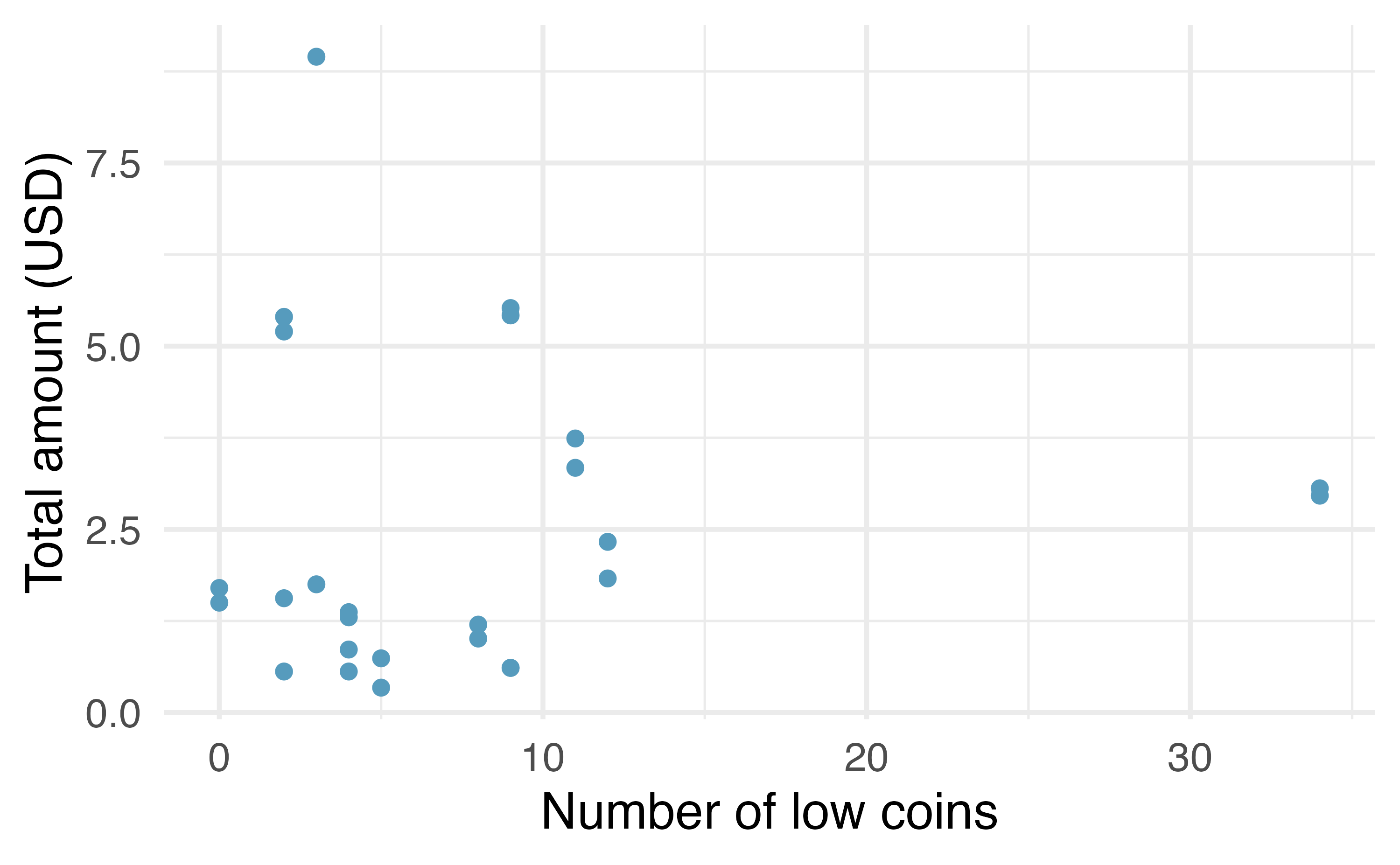
The collected data is given in Figure 25.5 and shows that the total_amount of money is more highly correlated with the total number_of_coins than it is with the number_of_low_coins.
Figure25.5.Two plots describing the total amount of money (USD) as a function of the total number of coins or low coins. As you might expect, the total amount of money is more highly positively correlated with the total number of coins than with the number of low coins.
The \(b_1 = 0.13\) coefficient has a small p-value associated with it, suggesting we would not have seen data like this if number_of_coins and total_amount of money were not linearly related.
The \(b_1 = 0.02\) coefficient has a large p-value associated with it, suggesting we could easily have seen data like ours even if the number_of_low_coins and total_amount of money are not at all linearly related.
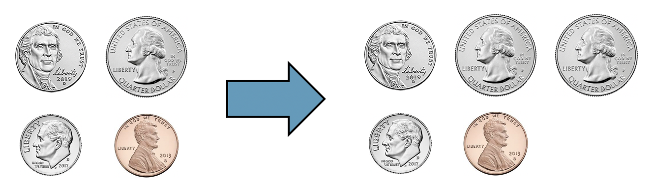
Two samples of coins with the same number of low coins (3), but a different number of total coins (4 vs 5) and a different total amount ($0.41 vs $0.66).
Two samples of coins with the same total number of coins (4), but a different number of low coins (3 vs 4) and a different total amount ($0.41 vs $0.17).
Using both the total number_of_coins and the number_of_low_coins as predictor variables, Table 25.16 provides the least squares estimates of both coefficients as 0.21 and -0.16.
A coefficient interpretation always indicates a change in one variable while keeping the other variable(s) constant. For every additional coin in the dish while the number_of_low_coins stays constant, we would predict that the student had US$0.21 more. Re-considering the phrase "every additional coin in the dish while the number of low coins stays constant" makes us realize that each increase is a single additional quarter (larger samples sizes would have led to a \(b_1\) coefficient closer to 0.25 because of the deterministic relationship described here).
For every additional low coin in the dish while the total number_of_coins stays constant, we would predict that the student had US$0.16 less. Re-considering the phrase "every additional low coin in the dish while the number of total coins stays constant" makes us realize that a quarter is being swapped out for a penny, nickel, or dime.
Considering the coefficients across Table 25.8, Table 25.10, and Table 25.16 within the context and knowledge we have of US coins allows us to understand the correlation between variables and why the signs of the coefficients would change depending on the model. Note also, however, that the p-value for the number_of_low_coins coefficient changed from Table 25.10 to Table 25.16. It makes sense that the variable describing the number_of_low_coins provides more information about the total_amount of money when it is part of a model which also includes the total number_of_coins than it does when it is used as a single variable in a simple linear regression model.
When working with multiple regression models, interpreting the model coefficients is not always as straightforward as it was with the coin example. However, we encourage you to always think carefully about the variables in the model, consider how they might be correlated among themselves, and work through different models to see how using different sets of variables might produce different relationships for predicting the response variable of interest.
Multicollinearity happens when the predictor variables are correlated within themselves. When the predictor variables themselves are correlated, the coefficients in a multiple regression model can be difficult to interpret.
Although diving into the details are beyond the scope of this text, we will provide one more reflection about multicollinearity. If the predictor variables have some degree of correlation, it can be quite difficult to interpret the value of the coefficient or evaluate whether the variable is a statistically discernible predictor of the outcome. However, even a model that suffers from high multicollinearity will likely lead to unbiased predictions of the response variable. So if the task at hand is only to do prediction (and not to interpret coefficients), multicollinearity is likely to not cause you substantial problems.
In Section 25.1, p-values were calculated on each of the model coefficients. The p-value gives a sense of which variables are important to the model; however, a more extensive treatment of variable selection is warranted in a follow-up course or textbook. Here, we use cross-validationprediction error to focus on which variable(s) are important for predicting the response variable of interest. In general, linear models are also used to make predictions of individual observations. In addition to model building, cross-validation provides a method for generating predictions that are not overfit to the particular dataset at hand. We continue to encourage you to take up further study on the topic of cross-validation, as it is among the most important ideas in modern data analysis, and we are only able to scratch the surface here.
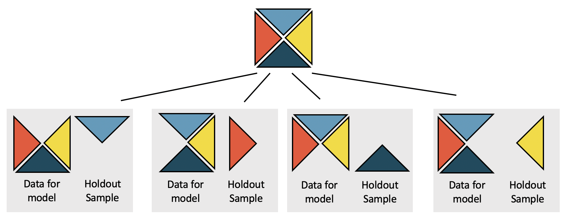
Cross-validation is a computational technique which removes some observations before a model is run, then assesses the model accuracy on the held-out sample. By removing some observations, we provide ourselves with an independent evaluation of the model (that is, the removed observations do not contribute to finding the parameters which minimize the least squares equation). Cross-validation can be used in many different ways (as an independent assessment), and here we will just scratch the surface with respect to one way the technique can be used to compare models. See Figure 25.17 for a visual representation of the cross-validation process.
Figure25.17.The dataset is broken into k folds (here k = 4). One at a time, a model is built using k-1 of the folds, and predictions are calculated on the single held out sample which will be completely independent of the model estimation.
Our goal in this section is to compare two different regression models which both seek to predict the mass of an individual penguin in grams. The observations of three different penguin species include measurements on body size and sex. The data were collected by Dr. Kristen Gorman and the Palmer Station, Antarctica LTER as part of the Long Term Ecological Research Network. Although not exactly aligned with this research project, you might be able to imagine a setting where the dimensions of the penguin are known (through, for example, aerial photographs) but the mass is not known. The first model predicts body_mass_g by using only the bill_length_mm, a variable denoting the length of a penguin’s bill, in mm. The second model predicts body_mass_g by using bill_length_mm, bill_depth_mm, flipper_length_mm, sex, and species.
The predicted error (also previously called the residual) is the difference between the observed value and the predicted value (from the regression model).
The presentation below (see the comparison of Figure 25.25 and Figure 25.28) shows that the model with more variables predicts body_mass_g with much smaller errors (predicted minus actual body mass) than the model which uses only bill_length_g. We have deliberately used a model that intuitively makes sense (the more body measurements, the more predictable mass is). However, in many settings, it is not obvious which variables or which models contribute most to accurate predictions. Cross-validation is one way to get accurate independent predictions with which to compare different models.
Subsection25.3.1Comparing two models to predict body mass in penguins
The question we will seek to answer is whether the predictions of body_mass_g are substantially better when bill_length_mm, bill_depth_mm, flipper_length_mm, sex, and species are used in the model, as compared with a model on bill_length_mm only.
We refer to the model given with only bill_length_mm as the smaller model. It is seen in Table 25.20 with coefficient estimates of the parameters as well as standard errors and p-values. We refer to the model given with bill_length_mm, bill_depth_mm, flipper_length_mm, sex, and species as the larger model. It is seen in Table 25.22 with coefficient estimates of the parameters as well as standard errors and p-values. Given what we know about high correlations between body measurements, it is somewhat unsurprising that all of the variables have low p-values, suggesting that each variable is a statistically discernible predictor of body_mass_g, given all other variables in the model. However, in this section, we will go beyond the use of p-values to consider independent predictions of body_mass_g as a way to compare the smaller and larger models.
Table25.22.Least squares estimates of the larger regression model predicting body_mass_g from bill_length_mm, bill_depth_mm, flipper_length_mm, sex, and species.
In order to compare the smaller and larger models in terms of their ability to predict penguin mass, we need to build models that can provide independent predictions based on the penguins in the holdout samples created by cross-validation. To reiterate, each of the predictions that (when combined together) will allow us to distinguish between the smaller and larger are independent of the data which were used to build the model.
In this example, using cross-validation, we remove one quarter of the data before running the least squares calculations. Then the least squares model is used to predict the body_mass_g of the penguins in the holdout sample. Here we use a 4-fold cross-validation (meaning that one quarter of the data is removed each time) to produce four different versions of each model (other times it might be more appropriate to use 2-fold or 10-fold or even run the model separately after removing each individual data point one at a time).
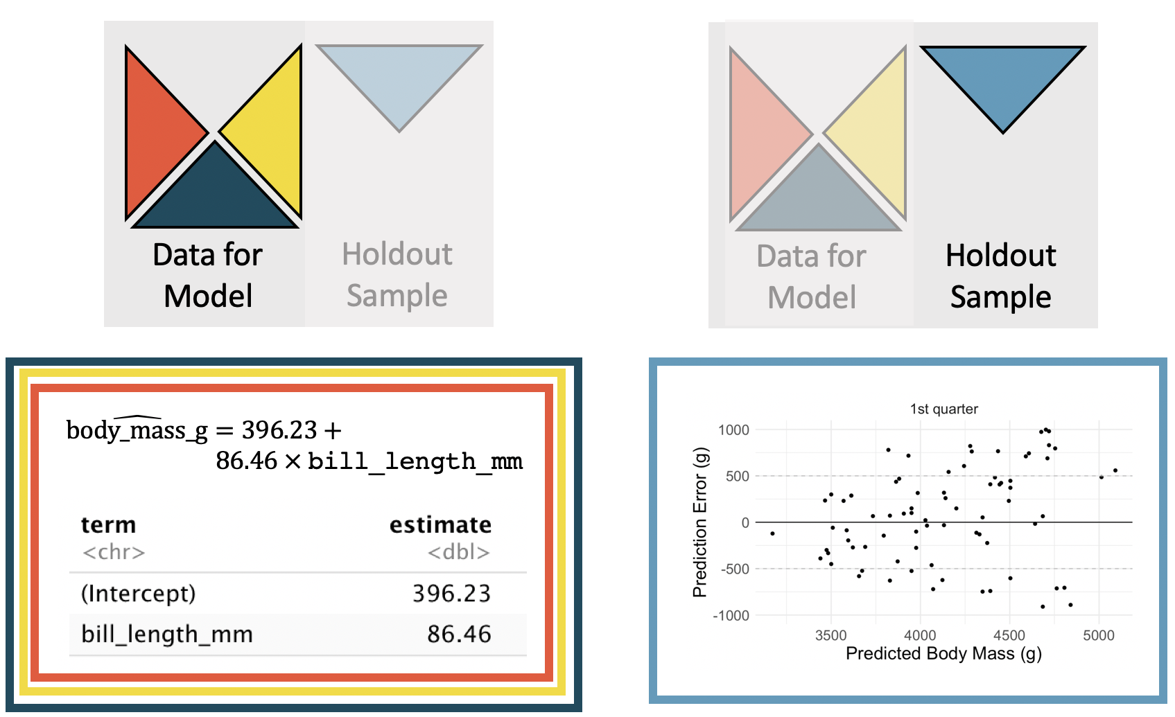
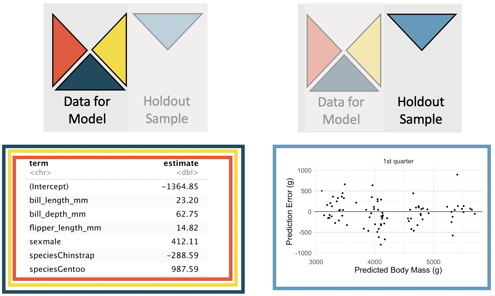
Figure 25.23 displays how a model is fit to 3/4 of the data (note the slight differences in coefficients as compared to Table 25.20), and then predictions are made on the holdout sample.
Figure25.23.The smaller model. The coefficients are estimated using the least squares model on 3/4 of the dataset with only a single predictor variable. Predictions are made on the remaining 1/4 of the observations. The y-axis in the scatterplot represents the residual, true observed value minus the predicted value. Note that the predictions are independent of the estimated model coefficients.
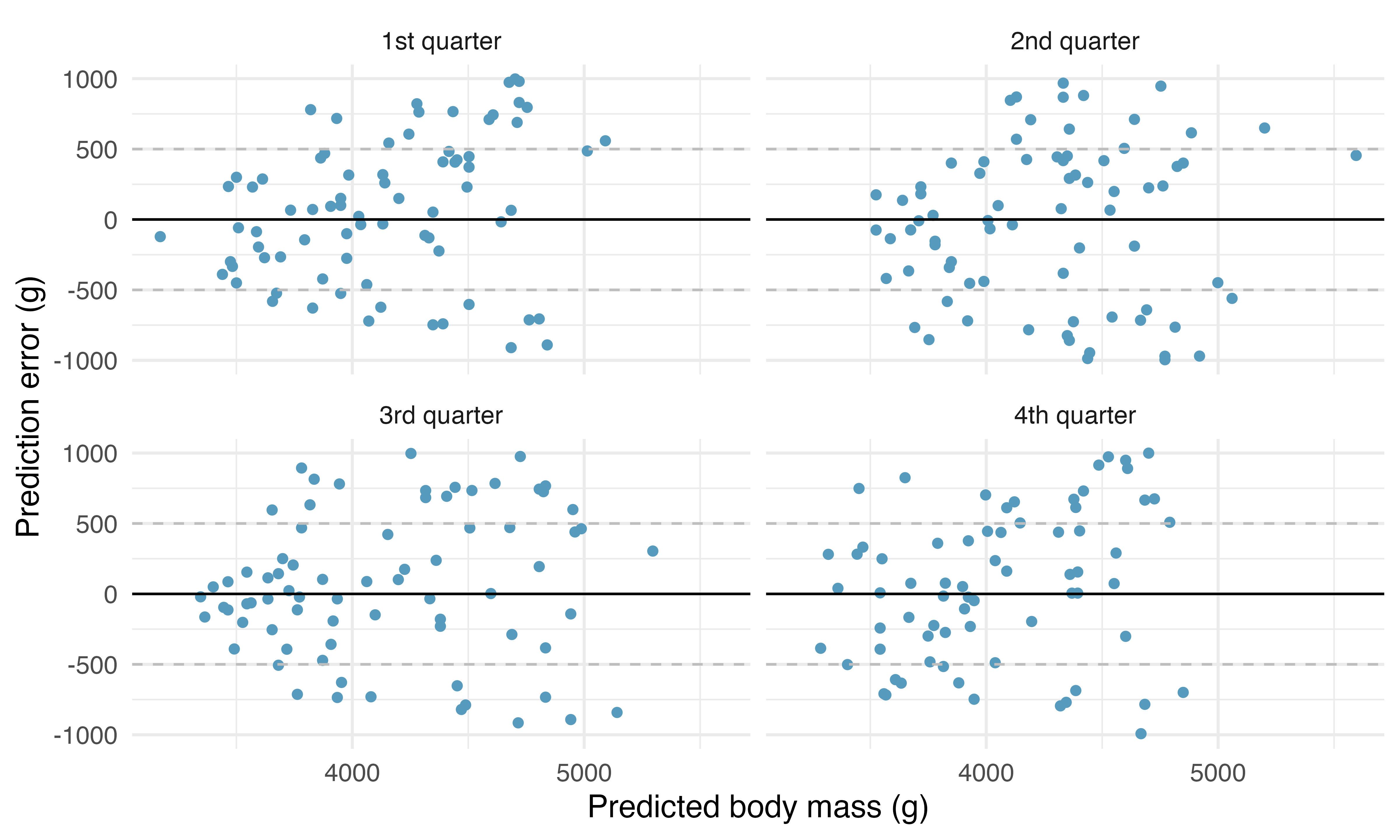
By repeating the process for each holdout quarter sample, the residuals from the model can be plotted against the predicted values. We see that the predictions are scattered which shows a good model fit but that the prediction errors vary \(\pm\) 1,000 g of the true body mass.
Figure25.25.The smaller model. One quarter at a time, the data were removed from the model building, and the body mass of the removed penguins was predicted. The least squares regression model was fit independently of the removed penguins. The predictions of body mass are based on bill length only. The x-axis represents the predicted value, the y-axis represents the error, the difference between predicted value and actual value.
The cross-validation SSE is the sum of squared error associated with the predictions. Let \(\hat{y}_{cv,i}\) be the prediction for the \(i^{th}\) observation where the \(i^{th}\) observation was in the hold-out fold and the other three folds were used to create the linear model. For the model using only bill_length_mm to predict body_mass_g, the CV SSE is 141,552,822.
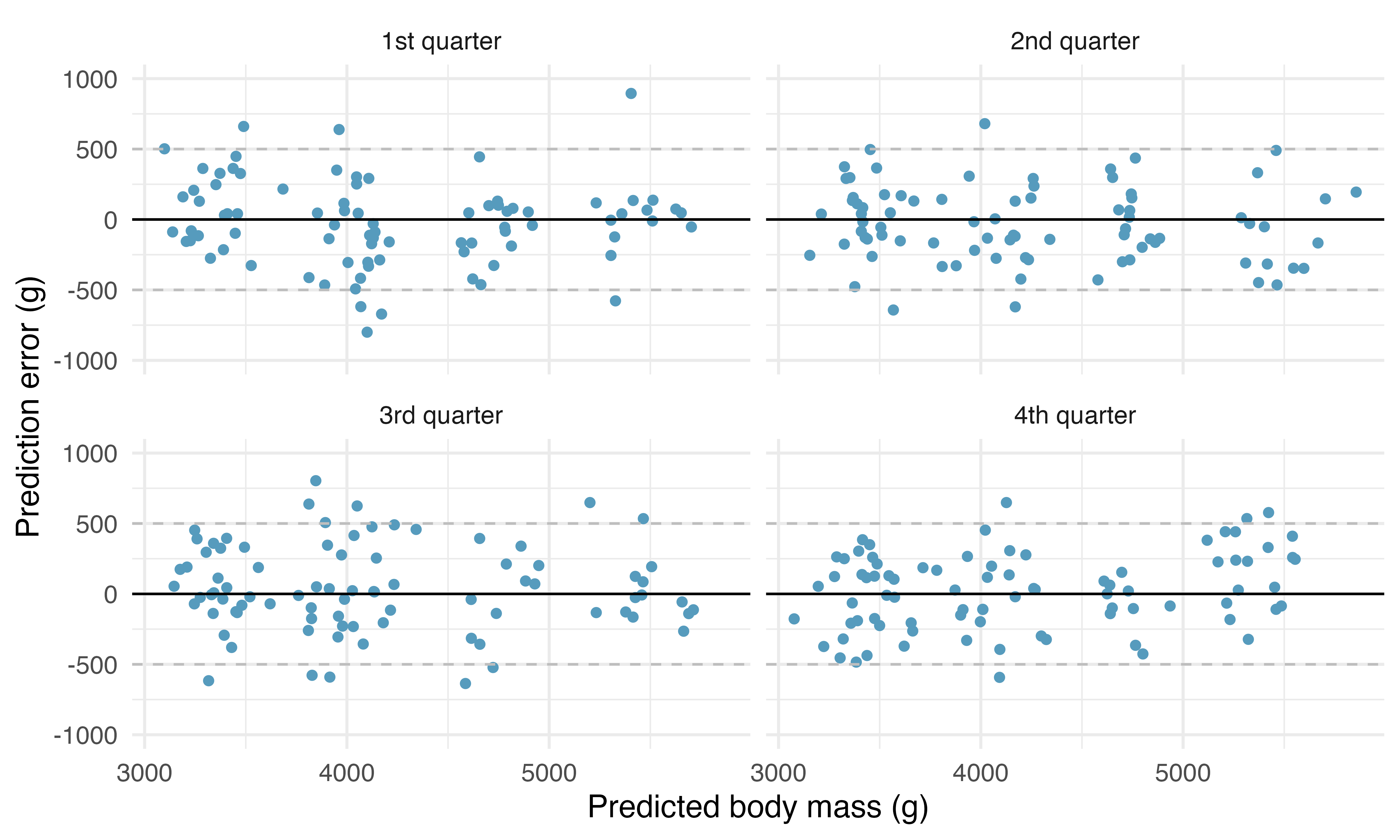
The same process is repeated for the larger number of explanatory variables. Note that the coefficients estimated for the first cross-validation model (in Figure 25.26) are slightly different from the estimates computed on the entire dataset (seen in Table 25.22). Figure 25.26 displays the cross-validation process for the multivariable model with a full set of residual plots given in Figure 25.28.Note that the residuals are mostly within \(\pm\) 500g, providing much more precise predictions for the independent body mass values of the individual penguins.
Figure25.26.The larger model. The coefficients are estimated using the least squares model on 3/4 of the dataset with the five specified predictor variables. Predictions are made on the remaining 1/4 of the observations. The y-axis in the scatterplot represents the residual, true observed value minus the predicted value. Note that the predictions are independent of the estimated model coefficients.
Figure25.28.The larger model. One quarter at a time, the data were removed from the model building, and the body mass of the removed penguins was predicted. The least squares regression model was fit independently of the removed penguins. The predictions of body mass are based on the set of five variables described in Table 25.22. The x-axis represents the predicted value, the y-axis represents the error, the difference between predicted value and actual value.
Figure 25.25 shows that the independent predictions are centered around the true values (i.e., errors are centered around zero), but that the predictions can be as much as 1,000 g off when using only bill_length_mm to predict body_mass_g. On the other hand, when using bill_length_mm, bill_depth_mm, flipper_length_mm, sex, and species to predict body_mass_g, the prediction errors seem to be about half as big, as seen in Figure 25.28. For the model using bill_length_mm, bill_depth_mm, flipper_length_mm, sex, and species to predict body_mass_g, the CV SSE is 27,728,698 (as compared to a CV SSE of 141,552,822 for the smaller model). Consistent with visually comparing the two sets of residual plots, the sum of squared prediction errors is smaller for the model which uses more predictor variables. The model with more predictor variables seems like the better model (according to the cross-validated prediction errors criteria).
We have provided a very brief overview to and example of using cross-validation. Cross-validation is a computational approach to model building and model validation as an alternative to reliance on p-values. While p-values have a role to play in understanding model coefficients, throughout this text, we have continued to present computational methods that broaden statistical approaches to data analysis. Cross-validation will be used again in Chapter 26 with logistic regression. We encourage you to consider both standard inferential methods (such as p-values) and computational approaches (such as cross-validation) as you build and use multivariable models of all varieties.
Building on the modeling ideas from Chapter 8, we have now introduced methods for evaluating coefficients (based on p-values) and evaluating models (cross-validation). There are many important aspects to consider when working with multiple variables in a single model, and we have only glanced at a few topics. Remember, multicollinearity can make coefficient interpretation difficult. A topic not covered in this text but important for multiple regression models is interaction, and we hope that you learn more about how variables work together as you continue to build up your modeling skills.
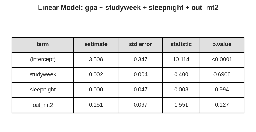
A survey of 55 Duke University students asked about their GPA (gpa), number of hours they study weekly (studyweek), number of hours they sleep nightly (sleepnight), and whether they go out more than two nights a week (out_mt2). We use these data to build a model predicting GPA from the other variables. Summary of the model is shown below. Note that out_mt2 is 1 if the student goes out more than two nights a week, and 0 otherwise. 3
The gpa data used in this exercise can be found in the openintro R package.
Calculate a 95% confidence interval for the coefficient of out_mt2 (go out more than two night a week) in the model, and interpret it in the context of the data.
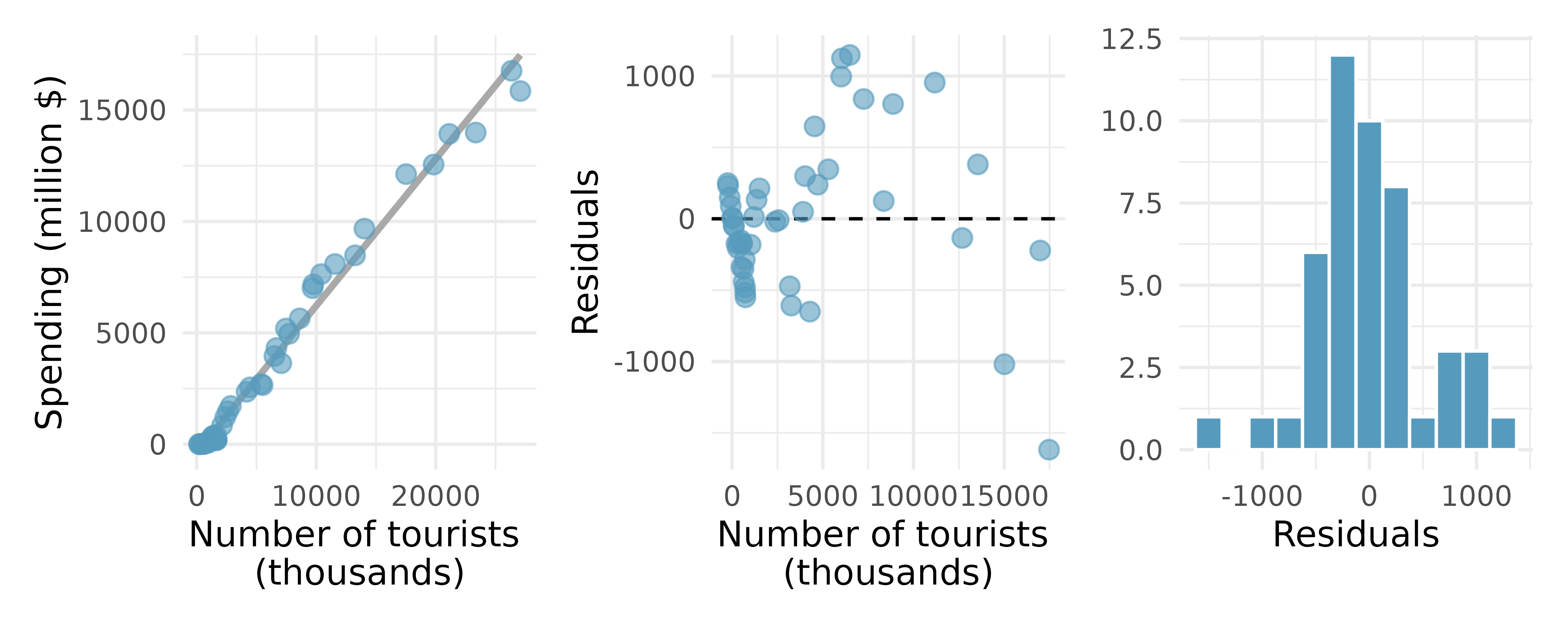
The Association of Turkish Travel Agencies reports the number of foreign tourists visiting Turkey and tourist spending by year. Three plots are provided: scatterplot showing the relationship between these two variables along with the least squares fit, residuals plot, and histogram of residuals. 4
The tourism data used in this exercise can be found in the openintro R package.
Do the data meet the LINE conditions required for fitting a least squares line? Use the scatterplot, the residuals plot, and the histogram to answer this question.
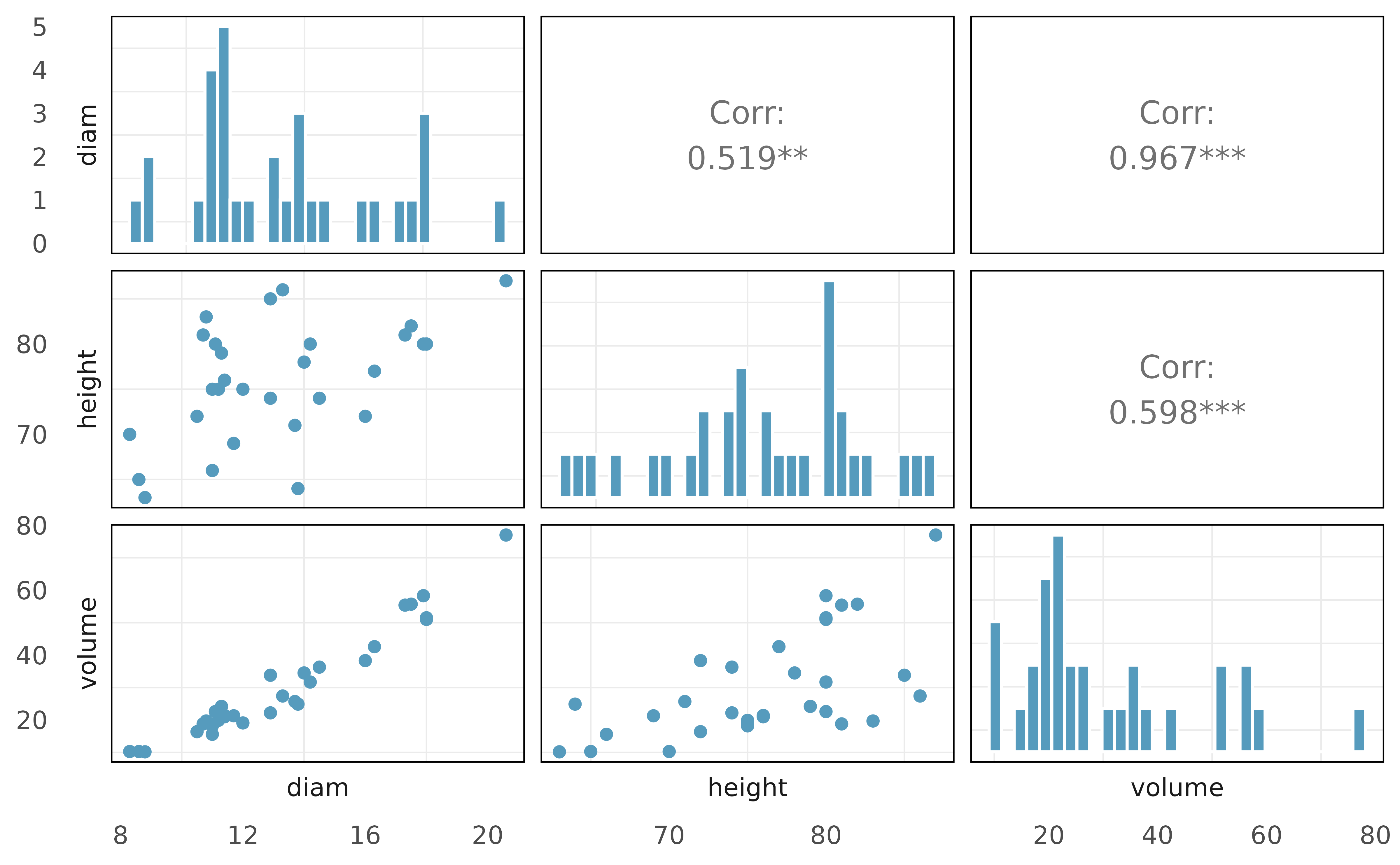
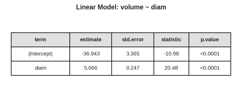
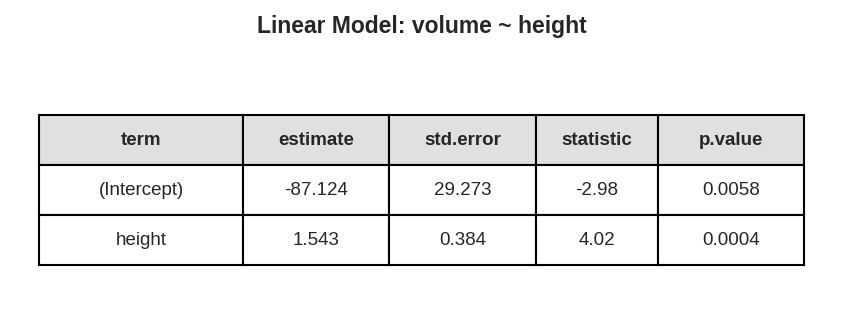
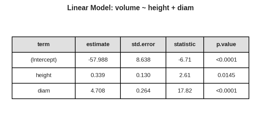
Timber yield is approximately equal to the volume of a tree, however, this value is difficult to measure without first cutting the tree down. Instead, other variables, such as height and diameter, may be used to predict a tree’s volume and yield. Researchers wanting to understand the relationship between these variables for black cherry trees collected data from 31 such trees in the Allegheny National Forest, Pennsylvania. Height is measured in feet, diameter in inches (at 54 inches above ground), and volume in cubic feet. 5
The cherry data used in this exercise can be found in the openintro R package.
The plots below display the distribution of each of these variables (on the diagonal) as well as provide information on the pairwise correlations between them.
There are three variables described in the figure, and each is paired with each other to create three different scatterplots. Rate the pairwise relationships from most correlated to least correlated.
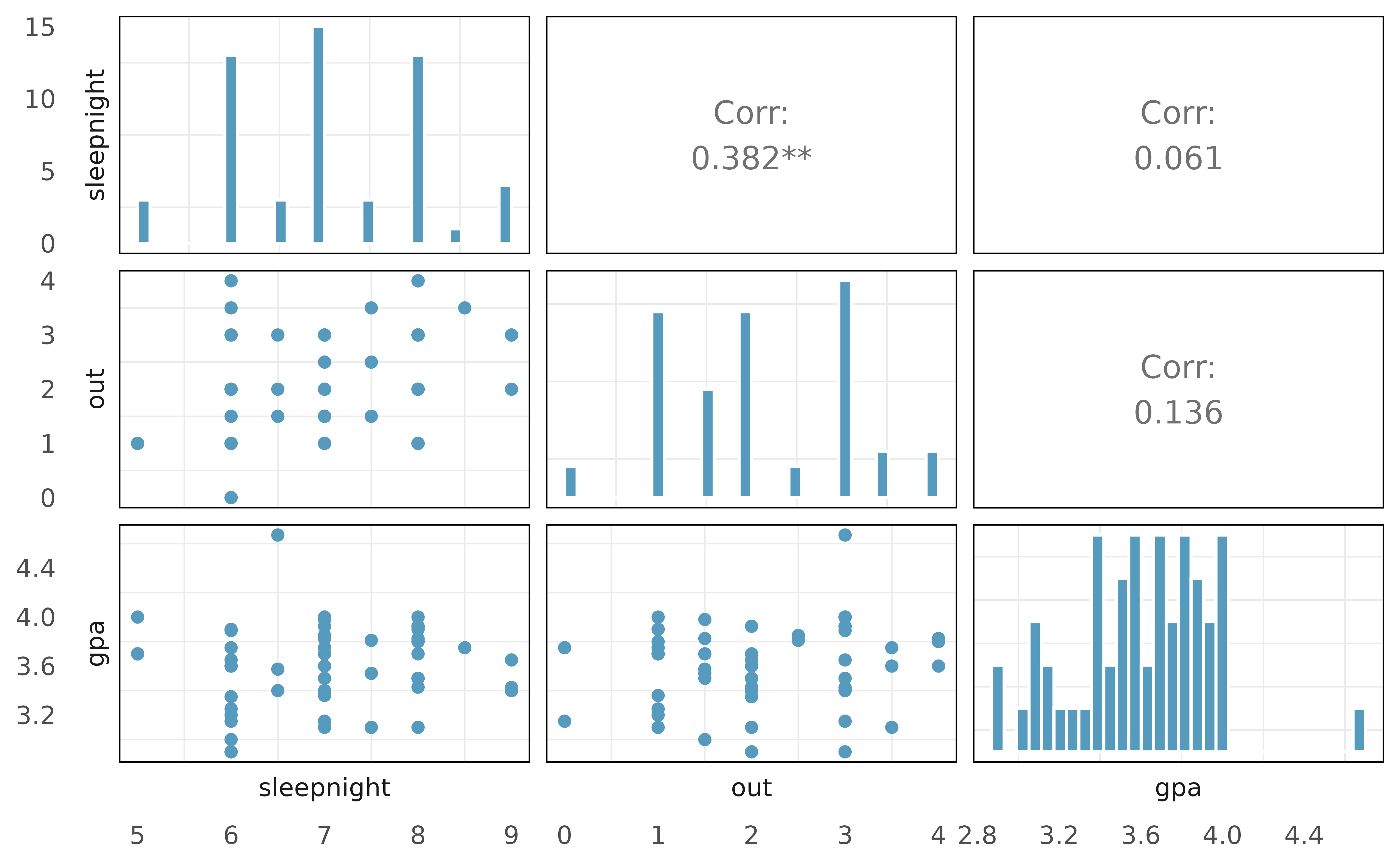
In this exercise we work with data from a survey of 55 Duke University students who were asked about their GPA, number of hours they sleep nightly, and number of nights they go out each week. The plots below display the distributions of each of these variables (on the diagonal) as well as their pairwise relationships and correlation coefficients.
There are three variables described in the figure, and each is paired with each other to create three different scatterplots. Rate the pairwise relationships from most correlated to least correlated.
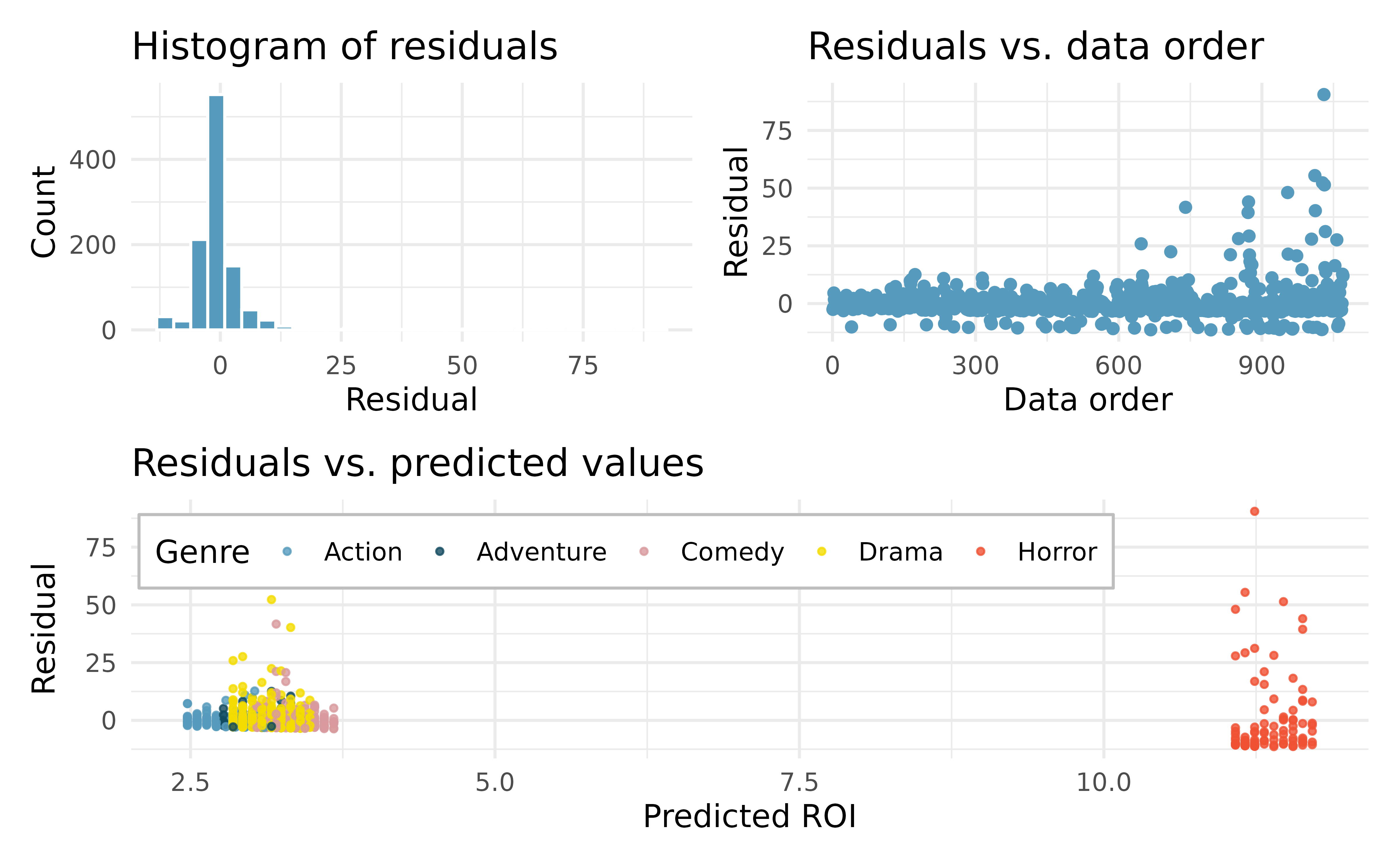
A FiveThirtyEight.com article reports that "Horror movies get nowhere near as much draw at the box office as the big-time summer blockbusters or action/adventure movies, but there’s a huge incentive for studios to continue pushing them out. The return-on-investment potential for horror movies is absurd." To investigate how the return-on-investment (ROI) compares between genres and how this relationship has changed over time, an introductory statistics student fit a linear regression model to predict the ratio of gross revenue of movies to the production costs from genre and release year for 1,070 movies released between 2000 and 2018. Using the plots given below, determine if this regression model is appropriate for these data. In particular, use the residual plot to check the LINE conditons.
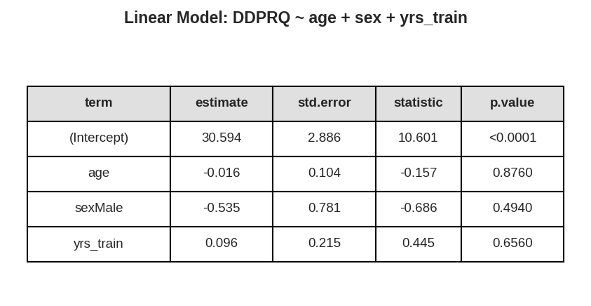
A study was conducted at a university outpatient primary care clinic in Switzerland to identify factors associated with difficult doctor-patient encounters. The data consist of 527 patient encounters, conducted by the 27 medical residents employed at the clinic. After each encounter, the attending physician completed two questionnaires: the Difficult Doctor Patient Relationship Questionnaire (DDPRQ-10) and the Patient’s Vulnerability Grid (PVG). A higher score on the DDPRQ-10 indicates a more difficult encounter. The maximum possible score is 60 and encounters with score 30 and higher are considered difficult. A model was fit to predict DDPRQ-10 score from features of the attending physician: age, sex (male or not), and years of training.
The intercept of the model is 30.594. What is the age, sex, and years of training of a physician whom this model would predict to have a DDPRQ-10 score of 30.594.
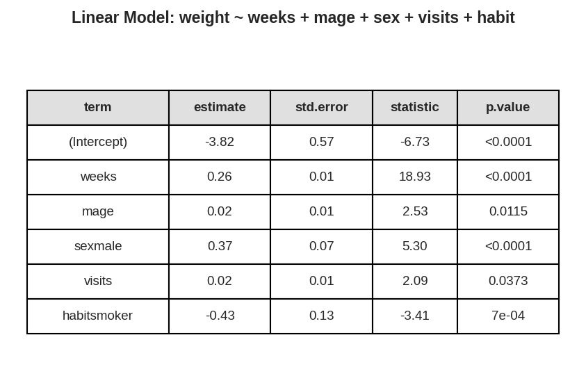
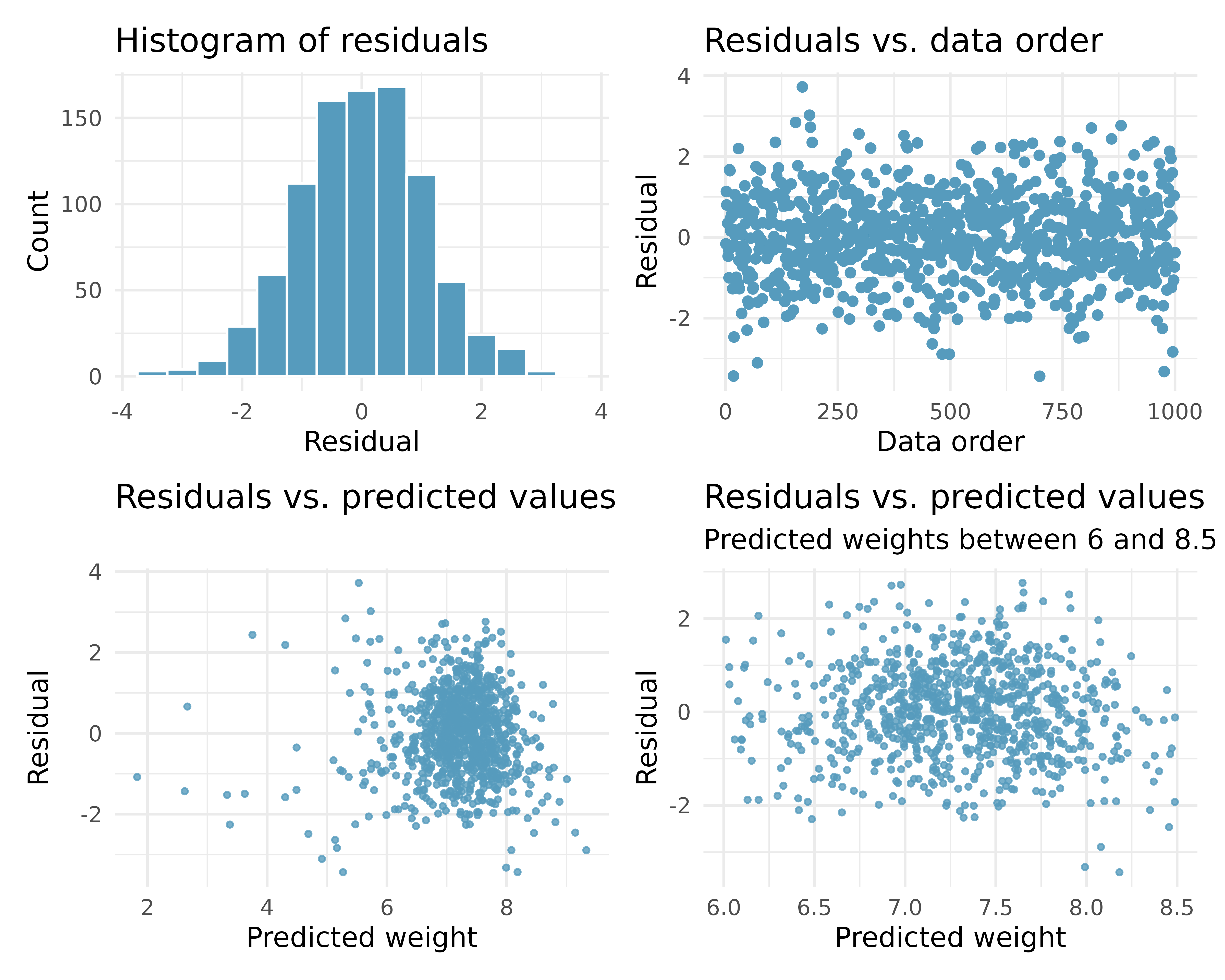
US Department of Health and Human Services, Centers for Disease Control and Prevention collect information on births recorded in the country. The data used here are a random sample of 1,000 births from 2014. Here, we study the relationship between smoking and weight of the baby. The variable smoke is coded 1 if the mother is a smoker, and 0 if not. The summary table below shows the results of a linear regression model for predicting the average birth weight of babies, measured in pounds, based on the smoking status of the mother. 6
The births14 data used in this exercise can be found in the openintro R package.
Determine if the conditions for doing inference based on mathematical models with these data are met using the diagnostic plots above. If not, describe how to proceed with the analysis.
Using the regression output, evaluate whether the true slope of habit (i.e., whether the mother is a smoker) is different than 0, given the other variables in the model. State the null and alternative hypotheses, report the p-value (using a mathematical model), and state your conclusion.
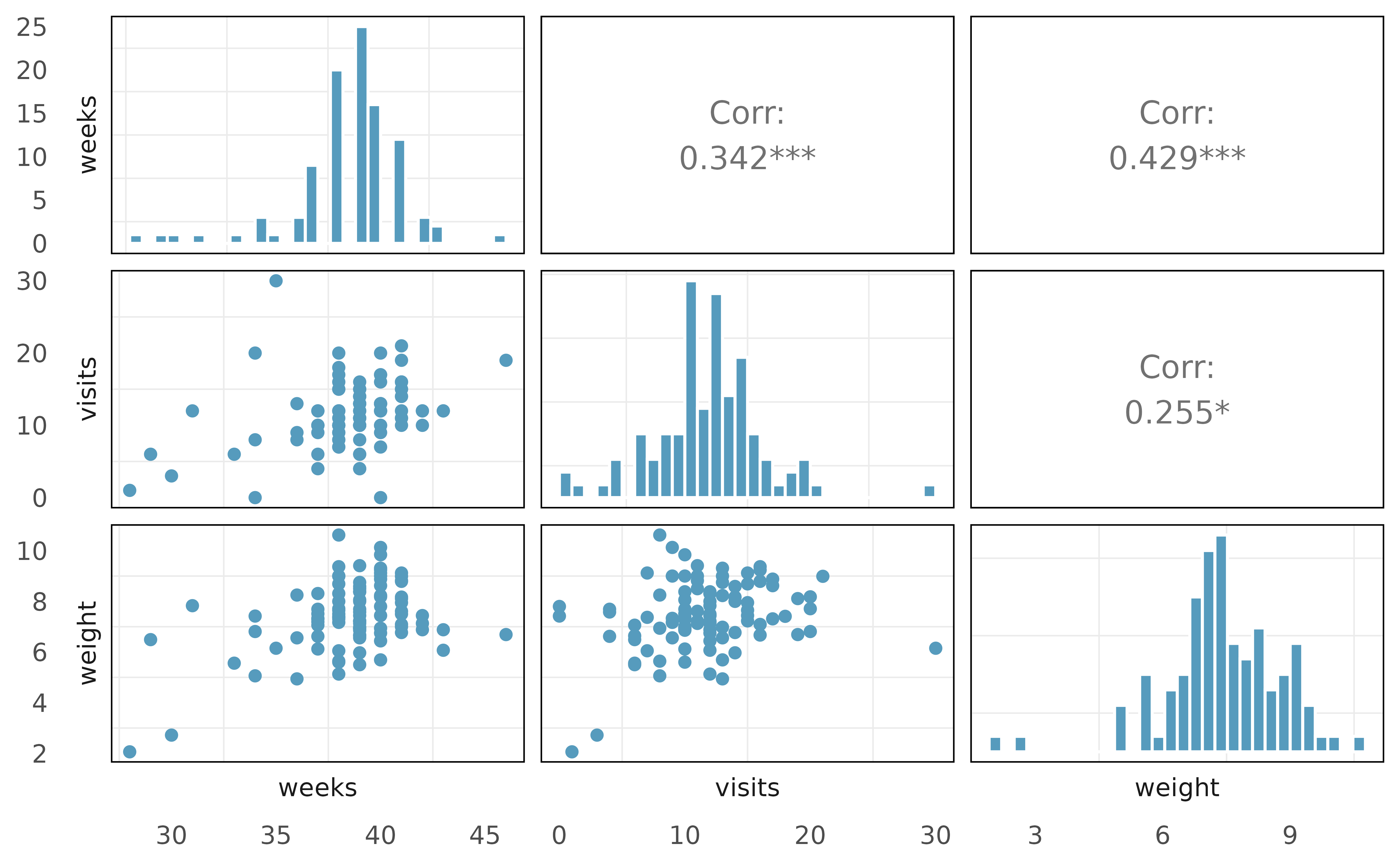
In this exercise we study the relationship between the weight of the baby and two explanatory variables: number of weeks of gestation and number of pregnancy hospital visits. The plots below display the distributions of each of these variables (on the diagonal) as well as their pairwise relationships and correlation coefficients.
There are three variables described in the figure, and each is paired with each other to create three different scatterplots. Rate the pairwise relationships from most correlated to least correlated.
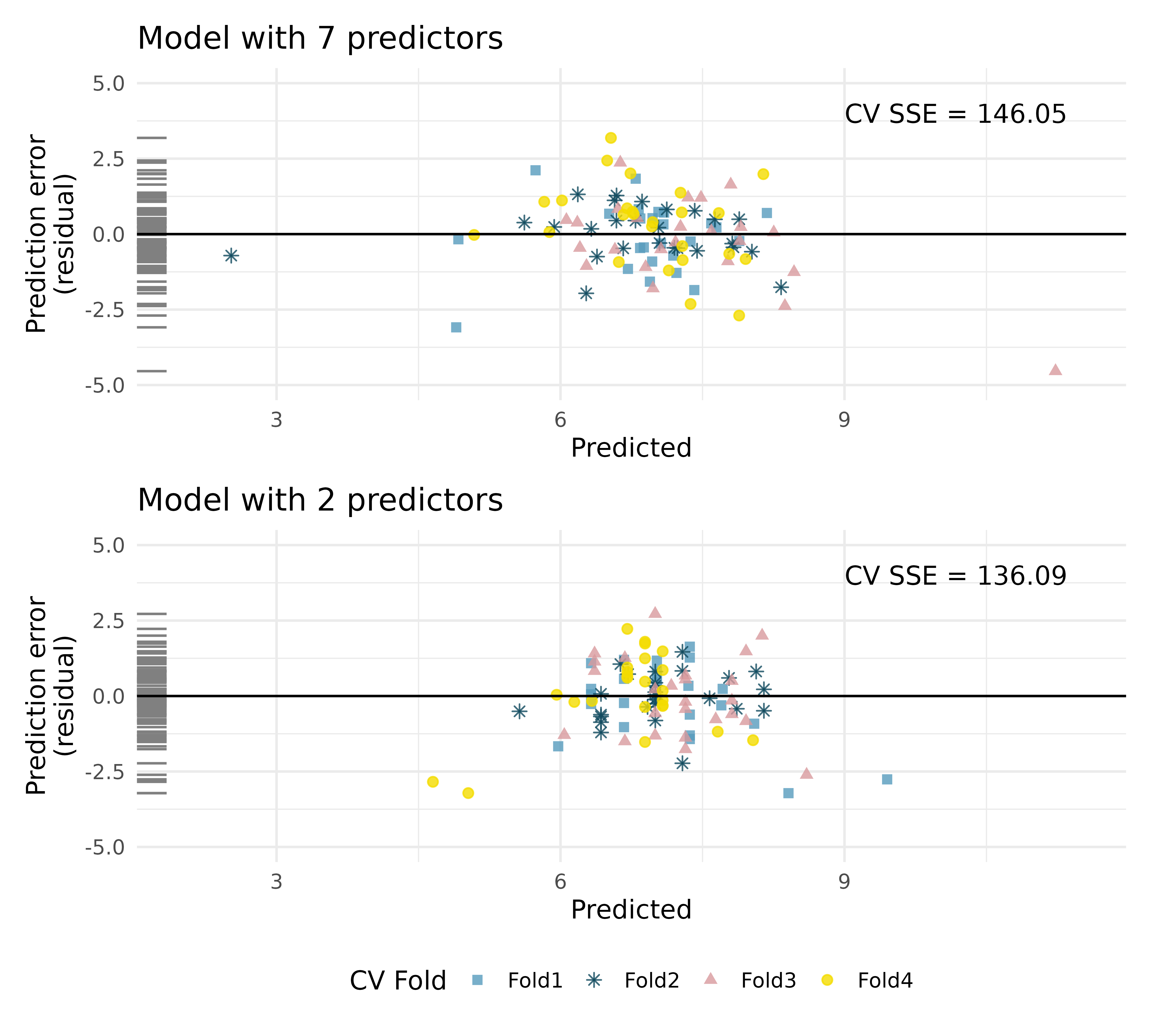
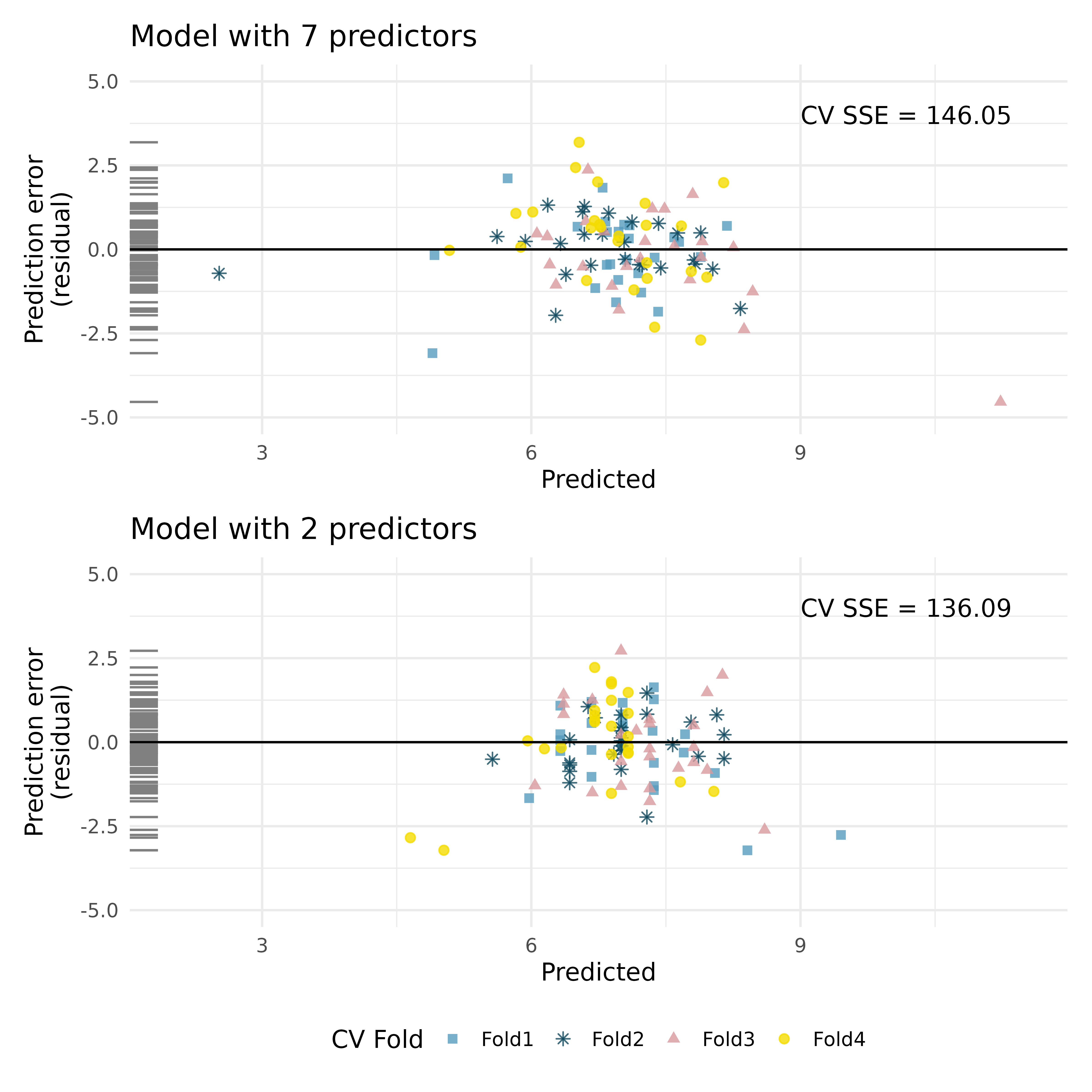
Using a random sample of 1,000 US births from 2014, we study the relationship between the weight of the baby and various explanatory variables. The plots below display prediction errors associated with two different models designed to predict weight of baby at birth; one model uses 7 predictors, one model uses 2 predictors. Using 4-fold cross-validation, the data were split into 4 folds. Three of the folds estimate the \(\beta_i\) parameters using \(b_i\text{,}\) and the model is applied to the held out fold for prediction. The process was repeated 4 times (each time holding out one of the folds).
For the plot on the top, for one of the cross-validation folds, how many coefficients were estimated in the linear model? For the plot on the bottom, for one of the cross-validation folds, how many coefficients were estimated in the linear model?
The Pioneer Valley Planning Commission (PVPC) collected data north of Chestnut Street in Florence, MA for ninety days from April 5, 2005 to November 15, 2005. Data collectors set up a laser sensor, with breaks in the laser beam recording when a rail-trail user passed the data collection station. 7
The RailTrail data used in this exercise can be found in the mosaicData R package.
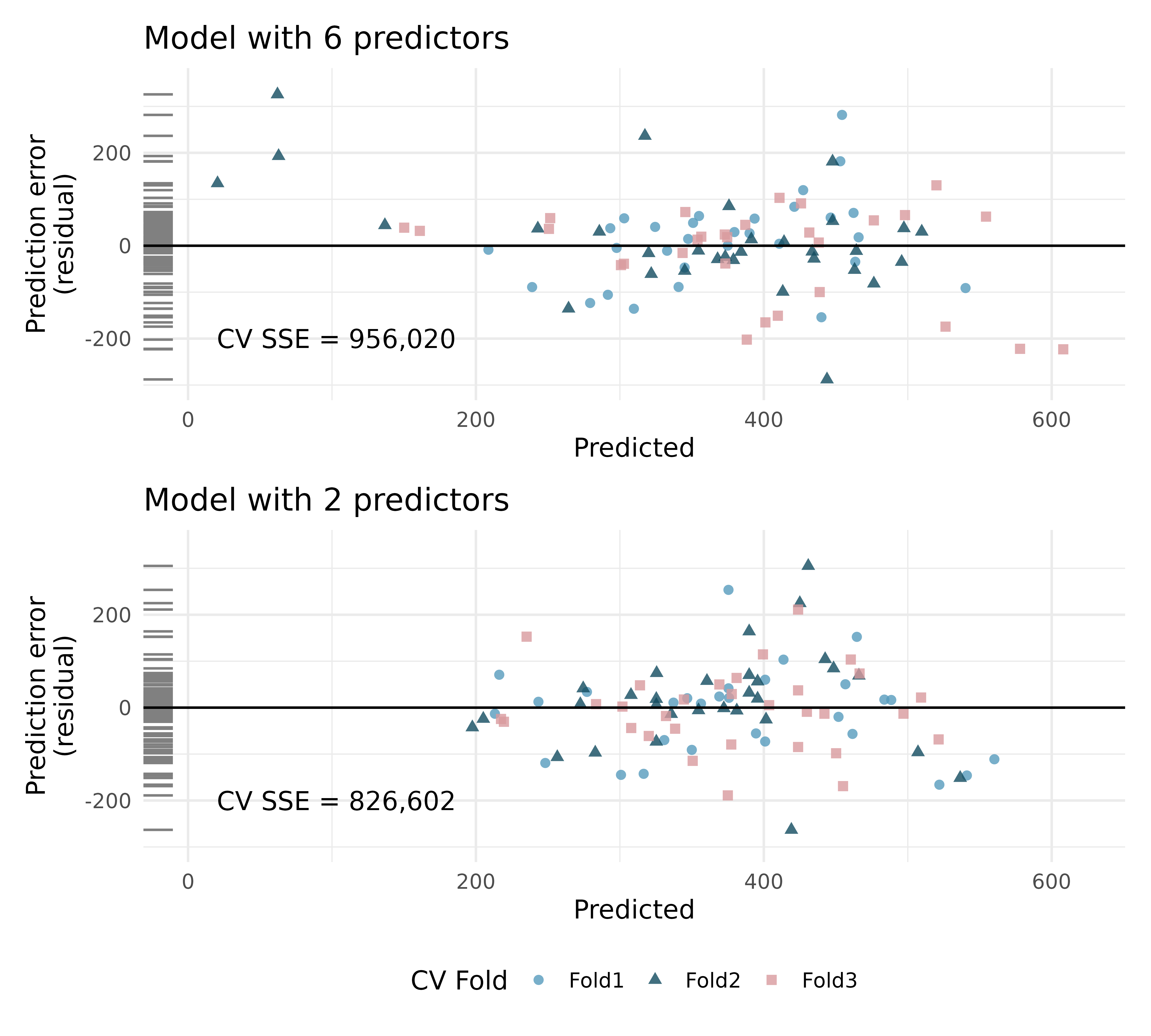
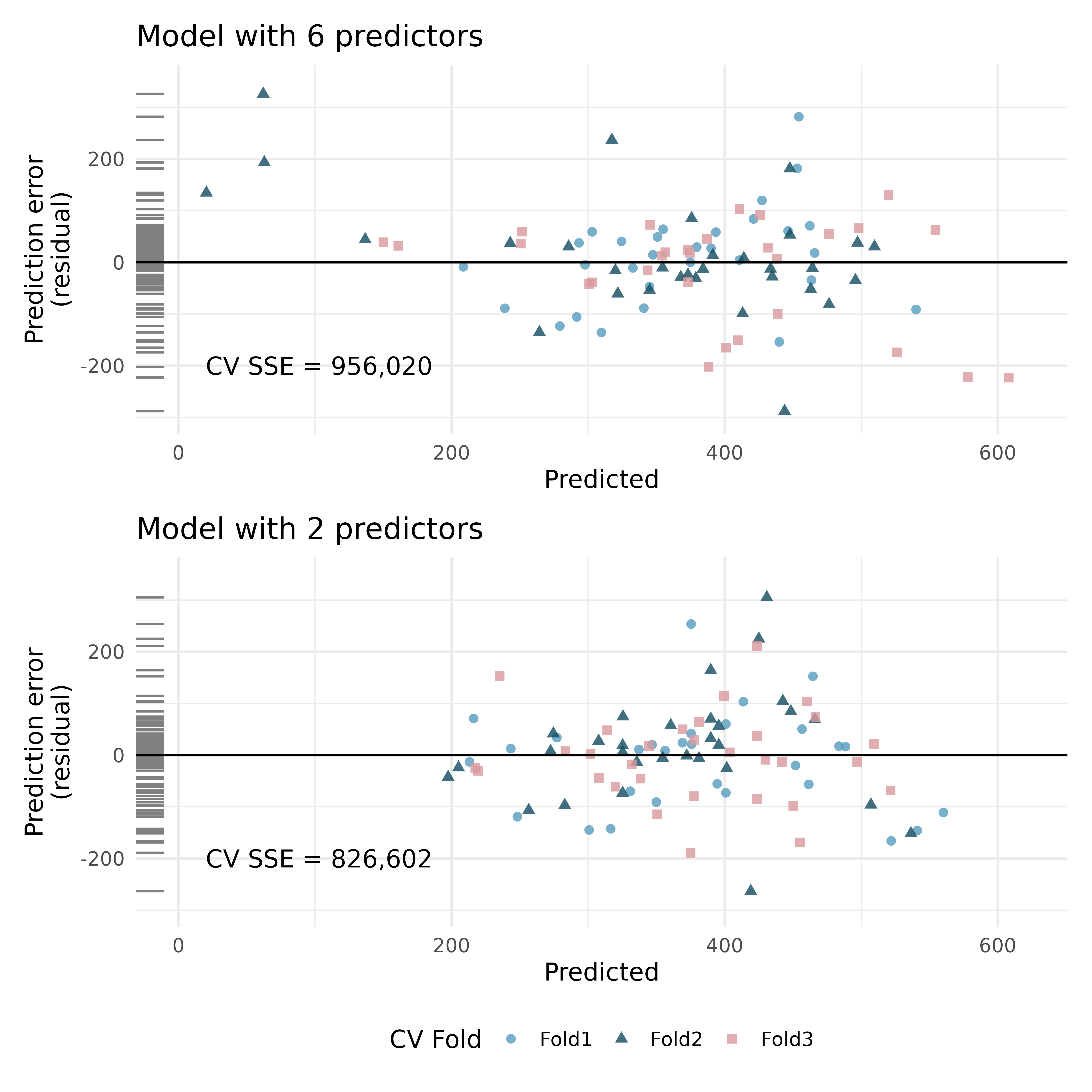
The plots below display prediction errors associated with two different models designed to predict the volume of riders on the RailTrail; one model uses 6 predictors, one model uses 2 predictors. Using 3-fold cross-validation, the data were split into 3 folds. Three of the folds estimate the \(\beta_i\) parameters using \(b_i\text{,}\) and the model is applied to the held out fold for prediction. The process was repeated 4 times (each time holding out one of the folds).
For the plot on the top, for one of the cross-validation folds, how many coefficients were estimated in the linear model? For the plot on the bottom, for one of the cross-validation folds, how many coefficients were estimated in the linear model?
11.Baby’s weight, cross-validation for model selection.
Using a random sample of 1,000 US births from 2014, we study the relationship between the weight of the baby and various explanatory variables. The plots below display prediction errors associated with two different models designed to predict weight of baby at birth; one model uses 7 predictors, one model uses 2 predictors. Using 4-fold cross-validation, the data were split into 4 folds. Three of the folds estimate the \(\beta_i\) parameters using \(b_i\text{,}\) and the model is applied to the held out fold for prediction. The process was repeated 4 times, each time holding out one of the folds.
12.RailTrail, cross-validation for model selection.
The Pioneer Valley Planning Commission (PVPC) collected data north of Chestnut Street in Florence, MA for ninety days from April 5, 2005 to November 15, 2005. Data collectors set up a laser sensor, with breaks in the laser beam recording when a rail-trail user passed the data collection station. The plots below display prediction errors associated with two different models designed to predict the volume of riders on the RailTrail; one model uses 6 predictors, one model uses 2 predictors. Using 3-fold cross-validation, the data were split into 3 folds. Three of the folds estimate the \(\beta_i\) parameters using \(b_i\text{,}\) and the model is applied to the held out fold for prediction. The process was repeated 4 times, each time holding out one of the folds.