Section 15.9 Create graphics with Asymptote
Asymptote (https://asymptote.sourceforge.io) is a powerful language for vector graphics. You may write and run Asymptote code in R Markdown with the
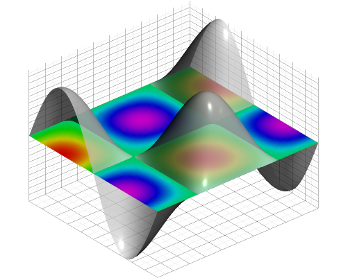
asy engine if you have installed Asymptote (see its website for instructions on the installation). Below is an example copied from the repository https://github.com/vectorgraphics/asymptote, and its output is shown in Figure 15.9.1:
```{asy, fig.cap='A 3D graph made with Asymptote.', cache=TRUE}
import graph3;
import grid3;
import palette;
settings.prc = false;

currentprojection=orthographic(0.8,1,2);
size(500,400,IgnoreAspect);

real f(pair z) {return cos(2*pi*z.x)*sin(2*pi*z.y);}

surface s=surface(f,(-1/2,-1/2),(1/2,1/2),50,Spline);

surface S=planeproject(unitsquare3)*s;
S.colors(palette(s.map(zpart),Rainbow()));
draw(S,nolight);
draw(s,lightgray+opacity(0.7));

grid3(XYZgrid);
```
Note that for PDF output, you may need some additional LaTeX packages, otherwise you may get an error that looks like this:
! LaTeX Error: File `ocgbase.sty' not found.
If such an error occurs, please see Section 1.3 for how to install the missing LaTeX packages.
In the
asy chunk above, we used the setting settings.prc = false. Without this setting, Asymptote generates an interactive 3D graph when the output format is PDF. However, the interactive graph can only be viewed in Acrobat Reader. If you use Acrobat Reader, you can interact with the graph. For example, you can rotate the 3D surface with your mouse.
Subsection 15.9.1 Generate data in R and read it in Asymptote
Now we show an example in which we first save data generated in R to a CSV file (below is an R code chunk):
x = seq(0, 5, l = 100)
y = sin(x)
writeLines(paste(x, y, sep = ','), 'sine.csv')
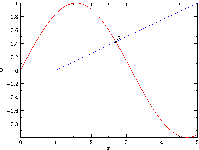
Then read it in Asymptote, and draw a graph based on the data as shown in Figure 15.9.2 (below is an
asy code chunk):
```{asy, fig.cap='Pass data from R to Asymptote to draw a graph.', cache=TRUE}
import graph;
size(400,300,IgnoreAspect);
settings.prc = false;

// import data from csv file
file in=input("sine.csv").line().csv();
real[][] a=in.dimension(0,0);
a=transpose(a);

// generate a path
path rpath = graph(a[0],a[1]);
path lpath = (1,0)--(5,1);

// find intersection
pair pA=intersectionpoint(rpath,lpath);

// draw all
draw(rpath,red);
draw(lpath,dashed + blue);
dot("$\delta$",pA,NE);
xaxis("$x$",BottomTop,LeftTicks);
yaxis("$y$",LeftRight,RightTicks);
```