Grid Algorithms for Hierarchical Models

Appendix H Grid Algorithms for Hierarchical Models

It is widely believed that grid algorithms are only practical for models with 1-3 parameters, or maybe 4-5 if you are careful. I’ve said so myself.

🔗

But recently I used a grid algorithm to solve the emitter-detector problem, and along the way I noticed something about the structure of the problem: although the model has two parameters, the data only depend on one of them. That makes it possible to evaluate the likelihood function and update the model very efficiently.

🔗

Many hierarchical models have a similar structure: the data depend on a small number of parameters, which depend on a small number of hyperparameters. I wondered whether the same method would generalize to more complex models, and it does.

🔗

As an example, in this notebook I’ll use a logitnormal-binomial hierarchical model to solve a problem with two hyperparameters and 13 parameters. The grid algorithm is not just practical; it’s substantially faster than MCMC.

🔗

The following are some utility functions I’ll use.

🔗

import matplotlib.pyplot as plt

def legend(**options):
    """Make a legend only if there are labels."""
    handles, labels = plt.gca().get_legend_handles_labels()
    if len(labels):
        plt.legend(**options)

def decorate(**options):
    plt.gca().set(**options)
    legend()
    plt.tight_layout()

from empiricaldist import Cdf

def compare_cdf(pmf, sample):
    pmf.make_cdf().step(label='grid')
    Cdf.from_seq(sample).plot(label='mcmc')
    print(pmf.mean(), sample.mean())
    decorate()

from empiricaldist import Pmf

def make_pmf(ps, qs, name):
    pmf = Pmf(ps, qs)
    pmf.normalize()
    pmf.index.name = name
    return pmf

Section H.1 Heart Attack Data

The problem I’ll solve is based on Chapter 10 of Probability and Bayesian Modeling; it uses data on death rates due to heart attack for patients treated at various hospitals in New York City.

🔗

We can use Pandas to read the data into a DataFrame.

🔗

import os

filename = 'DeathHeartAttackManhattan.csv'
if not os.path.exists(filename):
    !wget https://github.com/AllenDowney/BayesianInferencePyMC/raw/main/DeathHeartAttackManhattan.csv

import pandas as pd

df = pd.read_csv(filename)
df

                                        Hospital  Cases  Deaths  Death %
0                       Bellevue Hospital Center    129       4    3.101
1                         Harlem Hospital Center     35       1    2.857
2                            Lenox Hill Hospital    228      18    7.894
3                   Metropolitan Hospital Center     84       7    8.333
4                        Mount Sinai Beth Israel    291      24    8.247
5                           Mount Sinai Hospital    270      16    5.926
6                          Mount Sinai Roosevelt     46       6   13.043
7                         Mount Sinai St. Luke's    293      19    6.485
8                           NYU Hospitals Center    241      15    6.224
9                  NYP Hospital - Allen Hospital    105      13   12.381
10   NYP Hospital - Columbia Presbyterian Center    353      25    7.082
11  NYP Hospital - New York Weill Cornell Center    250      11    4.400
12                  NYP/Lower Manhattan Hospital     41       4    9.756

The columns we need are Cases, which is the number of patients treated at each hospital, and Deaths, which is the number of those patients who died.

🔗

data_ns = df['Cases'].values
data_ks = df['Deaths'].values

🔗

Section H.2 Solution with PyMC

Here’s a hierarchical model that estimates the death rate for each hospital and simultaneously estimates the distribution of rates across hospitals.

🔗

import pymc3 as pm

def make_model():
    with pm.Model() as model:
        mu = pm.Normal('mu', 0, 2)
        sigma = pm.HalfNormal('sigma', sigma=1)
        xs = pm.LogitNormal('xs', mu=mu, sigma=sigma, shape=len(data_ns))
        ks = pm.Binomial('ks', n=data_ns, p=xs, observed=data_ks)
    return model

%time model = make_model()
pm.model_to_graphviz(model)

CPU times: user 875 ms, sys: 51.7 ms, total: 927 ms
Wall time: 2.22 s

with model:
    pred = pm.sample_prior_predictive(1000)
    %time trace = pm.sample(500, target_accept=0.97)

Auto-assigning NUTS sampler...
Initializing NUTS using jitter+adapt_diag...
Multiprocess sampling (4 chains in 4 jobs)
NUTS: [xs, sigma, mu]
Sampling 4 chains for 1_000 tune and 500 draw iterations (4_000 + 2_000 draws total) took 8 seconds.
There were 2 divergences after tuning. Increase `target_accept` or reparameterize.
The acceptance probability does not match the target. It is 0.9060171753417431, but should be close to 0.97. Try to increase the number of tuning steps.
There was 1 divergence after tuning. Increase `target_accept` or reparameterize.
There were 7 divergences after tuning. Increase `target_accept` or reparameterize.
The acceptance probability does not match the target. It is 0.9337619072936738, but should be close to 0.97. Try to increase the number of tuning steps.
The estimated number of effective samples is smaller than 200 for some parameters.
CPU times: user 5.12 s, sys: 153 ms, total: 5.27 s
Wall time: 12.3 s

To be fair, PyMC doesn’t like this parameterization much (although I’m not sure why). One most runs, there are a moderate number of divergences. Even so, the results are good enough.

🔗

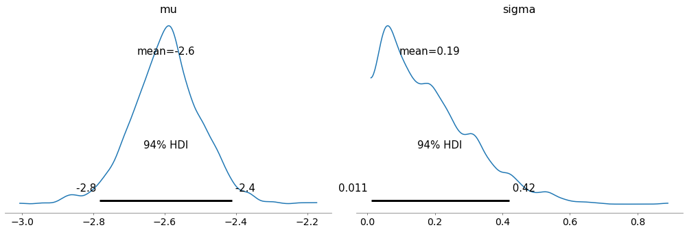
Here are the posterior distributions of the hyperparameters.

🔗

import arviz as az

with model:
    az.plot_posterior(trace, var_names=['mu', 'sigma'])

And we can extract the posterior distributions of the xs.

🔗

trace_xs = trace['xs'].transpose()
trace_xs.shape

(13, 2000)

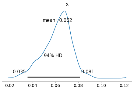
As an example, here’s the posterior distribution of x for the first hospital.

🔗

with model:
    az.plot_posterior(trace_xs[0])

🔗

Section H.3 The grid priors

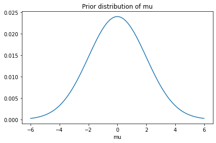
Now let’s solve the same problem using a grid algorithm. I’ll use the same priors for the hyperparameters, approximated by a grid with about 100 elements in each dimension.

🔗

import numpy as np
from scipy.stats import norm

mus = np.linspace(-6, 6, 101)
ps = norm.pdf(mus, 0, 2)
prior_mu = make_pmf(ps, mus, 'mu')

prior_mu.plot()
decorate(title='Prior distribution of mu')

from scipy.stats import logistic

sigmas = np.linspace(0.03, 3.6, 90)
ps = norm.pdf(sigmas, 0, 1)
prior_sigma = make_pmf(ps, sigmas, 'sigma')

prior_sigma.plot()
decorate(title='Prior distribution of sigma')

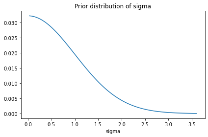
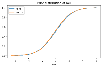
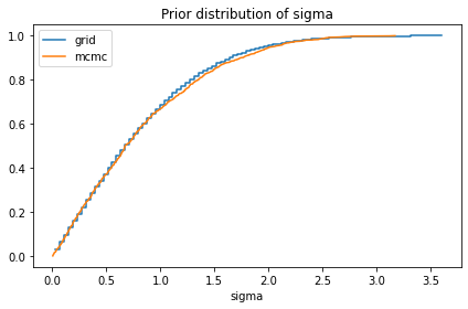
The following cells confirm that these priors are consistent with the prior samples from PyMC.

🔗

compare_cdf(prior_mu, pred['mu'])
decorate(title='Prior distribution of mu')

2.6020852139652106e-18 -0.06372282505953483

compare_cdf(prior_sigma, pred['sigma'])
decorate(title='Prior distribution of sigma')

0.8033718951689776 0.8244605687886865

🔗

Section H.4 The joint distribution of hyperparameters

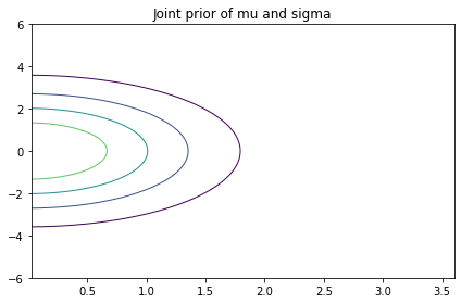
I’ll use make_joint to make an array that represents the joint prior distribution of the hyperparameters.

🔗

def make_joint(prior_x, prior_y):
    X, Y = np.meshgrid(prior_x.ps, prior_y.ps, indexing='ij')
    hyper = X * Y
    return hyper

prior_hyper = make_joint(prior_mu, prior_sigma)
prior_hyper.shape

(101, 90)

Here’s what it looks like.

🔗

import pandas as pd
from utils import plot_contour

plot_contour(pd.DataFrame(prior_hyper, index=mus, columns=sigmas))
decorate(title="Joint prior of mu and sigma")

🔗

Section H.5 Joint prior of hyperparameters and x

Now we’re ready to lay out the grid for x, which is the proportion we’ll estimate for each hospital.

🔗

xs = np.linspace(0.01, 0.99, 295)

For each pair of hyperparameters, we’ll compute the distribution of x.

🔗

from scipy.special import logit

M, S, X = np.meshgrid(mus, sigmas, xs, indexing='ij')
LO = logit(X)
LO.sum()

-6.440927791118156e-10

from scipy.stats import norm

%time normpdf = norm.pdf(LO, M, S)
normpdf.sum()

CPU times: user 69.6 ms, sys: 16.5 ms, total: 86.1 ms
Wall time: 84.9 ms
214125.5678798693

We can speed this up by computing skipping the terms that don’t depend on x.

🔗

%%time

z = (LO-M) / S
normpdf = np.exp(-z**2/2)

CPU times: user 26 ms, sys: 10.6 ms, total: 36.6 ms
Wall time: 35.1 ms

The result is a 3-D array with axes for mu, sigma, and x.

🔗

Now we need to normalize each distribution of x.

🔗

totals = normpdf.sum(axis=2)
totals.shape

(101, 90)

To normalize, we have to use a safe version of divide where 0/0 is 0.

🔗

def divide(x, y):
    out = np.zeros_like(x)
    return np.divide(x, y, out=out, where=(y!=0))

shape = totals.shape + (1,)
normpdf = divide(normpdf, totals.reshape(shape))
normpdf.shape

(101, 90, 295)

The result is an array that contains the distribution of x for each pair of hyperparameters.

🔗

Now, to get the prior distribution, we multiply through by the joint distribution of the hyperparameters.

🔗

def make_prior(hyper):

    # reshape hyper so we can multiply along axis 0
    shape = hyper.shape + (1,)
    prior = normpdf * hyper.reshape(shape)

    return prior

%time prior = make_prior(prior_hyper)
prior.sum()

CPU times: user 5.57 ms, sys: 0 ns, total: 5.57 ms
Wall time: 4.87 ms
0.999937781278039

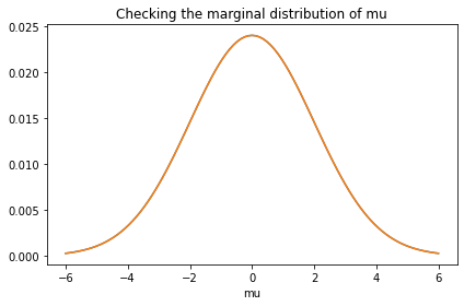
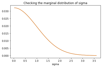
The result is a 3-D array that represents the joint prior distribution of mu, sigma, and x.

🔗

To check that it is correct, I’ll extract the marginal distributions and compare them to the priors.

🔗

def marginal(joint, axis):
    axes = [i for i in range(3) if i != axis]
    return joint.sum(axis=tuple(axes))

prior_mu.plot()
marginal_mu = Pmf(marginal(prior, 0), mus)
marginal_mu.plot()
decorate(title='Checking the marginal distribution of mu')

prior_sigma.plot()
marginal_sigma = Pmf(marginal(prior, 1), sigmas)
marginal_sigma.plot()
decorate(title='Checking the marginal distribution of sigma')

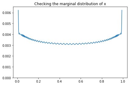
We didn’t compute the prior distribution of x explicitly; it follows from the distribution of the hyperparameters. But we can extract the prior marginal of x from the joint prior.

🔗

marginal_x = Pmf(marginal(prior, 2), xs)
marginal_x.plot()
decorate(title='Checking the marginal distribution of x',
         ylim=[0, np.max(marginal_x) * 1.05])

And compare it to the prior sample from PyMC.

🔗

pred_xs = pred['xs'].transpose()
pred_xs.shape

(13, 1000)

compare_cdf(marginal_x, pred_xs[0])
decorate(title='Prior distribution of x')

0.49996889063901967 0.4879934000104224

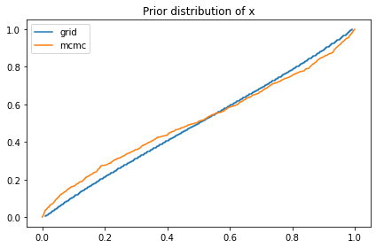
The prior distribution of x I get from the grid is a bit different from what I get from PyMC. I’m not sure why, but it doesn’t seem to affect the results much.

🔗

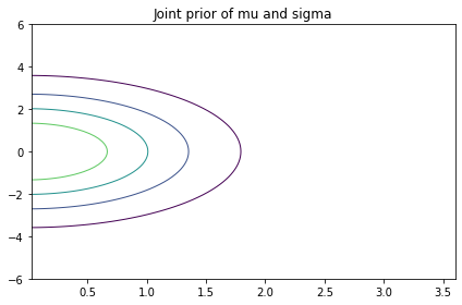
In addition to the marginals, we’ll also find it useful to extract the joint marginal distribution of the hyperparameters.

🔗

def get_hyper(joint):
    return joint.sum(axis=2)

hyper = get_hyper(prior)

plot_contour(pd.DataFrame(hyper,
                          index=mus,
                          columns=sigmas))
decorate(title="Joint prior of mu and sigma")

🔗

Section H.6 The Update

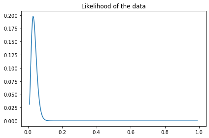
The likelihood of the data only depends on x, so we can compute it like this.

🔗

from scipy.stats import binom

data_k = data_ks[0]
data_n = data_ns[0]

like_x = binom.pmf(data_k, data_n, xs)
like_x.shape

(295,)

plt.plot(xs, like_x)
decorate(title='Likelihood of the data')

And here’s the update.

🔗

def update(prior, data):
    n, k = data
    like_x = binom.pmf(k, n, xs)
    posterior = prior * like_x
    posterior /= posterior.sum()
    return posterior

data = data_n, data_k
%time posterior = update(prior, data)

CPU times: user 11.6 ms, sys: 11.9 ms, total: 23.5 ms
Wall time: 7.66 ms

🔗

Section H.7 Serial updates

At this point we can do an update based on a single hospital, but how do we update based on all of the hospitals?

🔗

As a step toward the right answer, I’ll start with a wrong answer, which is to do the updates one at a time.

🔗

After each update, we extract the posterior distribution of the hyperparameters and use it to create the prior for the next update.

🔗

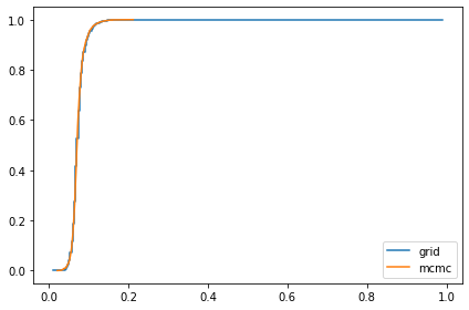
At the end, the posterior distribution of hyperparameters is correct, and the marginal posterior of x for the last hospital is correct, but the other marginals are wrong because they do not take into account data from subsequent hospitals.

🔗

def multiple_updates(prior, ns, ks):
    for data in zip(ns, ks):
        print(data)
        posterior = update(prior, data)
        hyper = get_hyper(posterior)
        prior = make_prior(hyper)
    return posterior

%time posterior = multiple_updates(prior, data_ns, data_ks)

(129, 4)
(35, 1)
(228, 18)
(84, 7)
(291, 24)
(270, 16)
(46, 6)
(293, 19)
(241, 15)
(105, 13)
(353, 25)
(250, 11)
(41, 4)
CPU times: user 185 ms, sys: 35.4 ms, total: 220 ms
Wall time: 172 ms

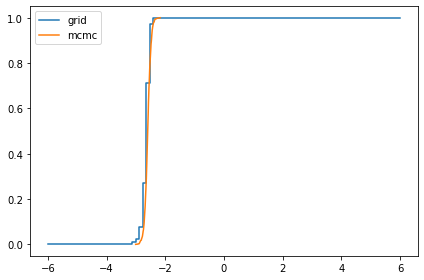
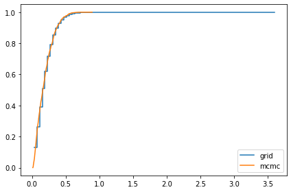
Here are the posterior distributions of the hyperparameters, compared to the results from PyMC.

🔗

marginal_mu = Pmf(marginal(posterior, 0), mus)
compare_cdf(marginal_mu, trace['mu'])

-2.6478808810110768 -2.5956645549514694

marginal_sigma = Pmf(marginal(posterior, 1), sigmas)
compare_cdf(marginal_sigma, trace['sigma'])

0.19272226451430116 0.18501785022543282

marginal_x = Pmf(marginal(posterior, 2), xs)
compare_cdf(marginal_x, trace_xs[-1])

0.07330826956150183 0.07297933578329886

🔗

Section H.8 Parallel updates

Doing updates one at time is not quite right, but it gives us an insight.

🔗

Suppose we start with a uniform distribution for the hyperparameters and do an update with data from one hospital. If we extract the posterior joint distribution of the hyperparameters, what we get is the likelihood function associated with one dataset.

🔗

The following function computes these likelihood functions and saves them in an array called hyper_likelihood.

🔗

def compute_hyper_likelihood(ns, ks):
    shape = ns.shape + mus.shape + sigmas.shape
    hyper_likelihood = np.empty(shape)

    for i, data in enumerate(zip(ns, ks)):
        print(data)
        n, k = data
        like_x = binom.pmf(k, n, xs)
        posterior = normpdf * like_x
        hyper_likelihood[i] = get_hyper(posterior)
    return hyper_likelihood

%time hyper_likelihood = compute_hyper_likelihood(data_ns, data_ks)

(129, 4)
(35, 1)
(228, 18)
(84, 7)
(291, 24)
(270, 16)
(46, 6)
(293, 19)
(241, 15)
(105, 13)
(353, 25)
(250, 11)
(41, 4)
CPU times: user 82 ms, sys: 55.2 ms, total: 137 ms
Wall time: 75.5 ms

We can multiply this out to get the product of the likelihoods.

🔗

%time hyper_likelihood_all = hyper_likelihood.prod(axis=0)
hyper_likelihood_all.sum()

CPU times: user 279 µs, sys: 0 ns, total: 279 µs
Wall time: 158 µs
1.685854062633571e-14

This is useful because it provides an efficient way to compute the marginal posterior distribution of x for any hospital. Here’s an example.

🔗

i = 3
data = data_ns[i], data_ks[i]
data

(84, 7)

Suppose we did the updates serially and saved this hospital for last. The prior distribution for the final update would reflect the updates from all previous hospitals, which we can compute by dividing out hyper_likelihood[i].

🔗

%time hyper_i = divide(prior_hyper * hyper_likelihood_all, hyper_likelihood[i])
hyper_i.sum()

CPU times: user 310 µs, sys: 147 µs, total: 457 µs
Wall time: 342 µs
4.3344287278716945e-17

We can use hyper_i to make the prior for the last update.

🔗

prior_i = make_prior(hyper_i)

And then do the update.

🔗

posterior_i = update(prior_i, data)

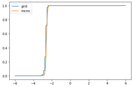
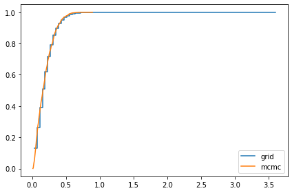
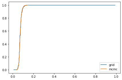
And we can confirm that the results are similar to the results from PyMC.

🔗

marginal_mu = Pmf(marginal(posterior_i, 0), mus)
marginal_sigma = Pmf(marginal(posterior_i, 1), sigmas)
marginal_x = Pmf(marginal(posterior_i, 2), xs)

compare_cdf(marginal_mu, trace['mu'])

-2.647880881011078 -2.5956645549514694

compare_cdf(marginal_sigma, trace['sigma'])

0.19272226451430124 0.18501785022543282

compare_cdf(marginal_x, trace_xs[i])

0.07245354421667904 0.07224440565018131

🔗

Section H.9 Compute all marginals

The following function computes the marginals for all hospitals and stores the results in an array.

🔗

def compute_all_marginals(ns, ks):
    shape = len(ns), len(xs)
    marginal_xs = np.zeros(shape)
    numerator = prior_hyper * hyper_likelihood_all

    for i, data in enumerate(zip(ns, ks)):
        hyper_i = divide(numerator, hyper_likelihood[i])
        prior_i = make_prior(hyper_i)
        posterior_i = update(prior_i, data)
        marginal_xs[i] = marginal(posterior_i, 2)

    return marginal_xs

%time marginal_xs = compute_all_marginals(data_ns, data_ks)

CPU times: user 184 ms, sys: 49.8 ms, total: 234 ms
Wall time: 173 ms

Here’s what the results look like, compared to the results from PyMC.

🔗

for i, ps in enumerate(marginal_xs):
    pmf = Pmf(ps, xs)
    plt.figure()
    compare_cdf(pmf, trace_xs[i])
    decorate(title=f'Posterior marginal of x for Hospital {i}',
             xlabel='Death rate',
             ylabel='CDF',
             xlim=[trace_xs[i].min(), trace_xs[i].max()])

0.06123636407822421 0.0617519291444324
0.06653003152551518 0.06643868288267936
0.07267383211481376 0.07250041300148316
0.07245354421667904 0.07224440565018131
0.07430385699796423 0.07433369435815212
0.06606326919655045 0.06646020352443961
0.07774639529896528 0.07776805141855801
0.06788483681522386 0.06807113157490664
0.06723306224279789 0.06735326167909643
0.08183332535205982 0.08115900598539395
0.07003760661997555 0.0704088595242495
0.06136130741477605 0.06159674913422137
0.07330826956150185 0.07297933578329886

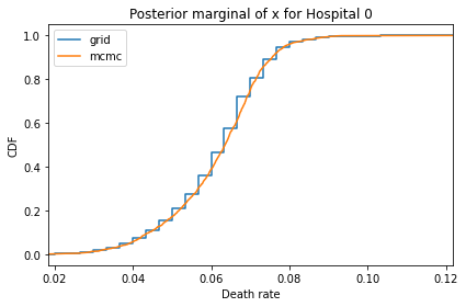
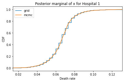
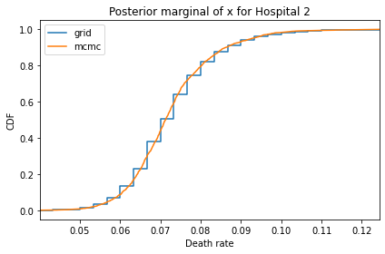
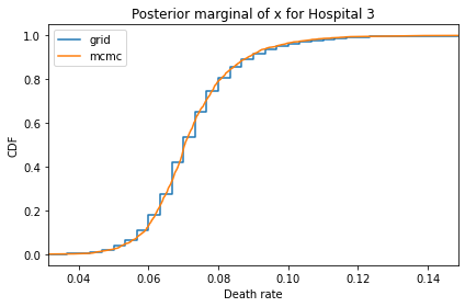
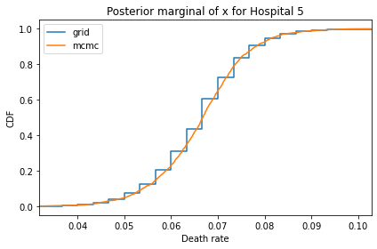
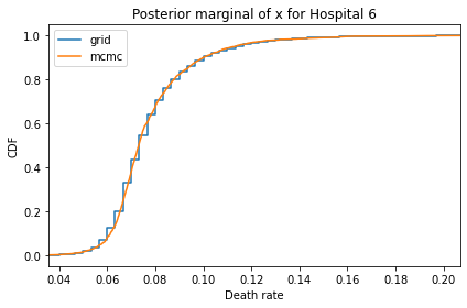
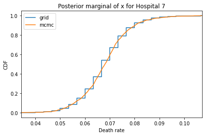
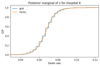
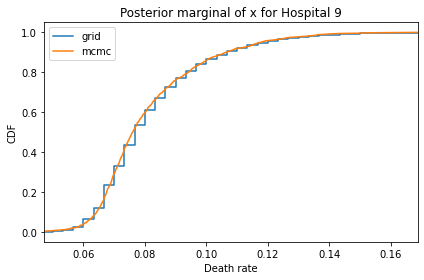
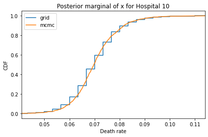
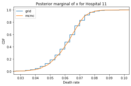
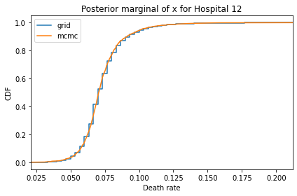
And here are the percentage differences between the results from the grid algorithm and PyMC. Most of them are less than 1%.

🔗

for i, ps in enumerate(marginal_xs):
    pmf = Pmf(ps, xs)
    diff = abs(pmf.mean() - trace_xs[i].mean()) / pmf.mean()
    print(diff * 100)

0.841926319383687
0.13730437329010417
0.23862662568368032
0.28865194761527047
0.04015586995533174
0.6008396688759207
0.027854821447936134
0.274427646029194
0.17878024931315142
0.8240155997142278
0.5300765148763152
0.38369736461746806
0.44869941709241024

The total time to do all of these computations is about 300 ms, compared to more than 10 seconds to make and run the PyMC model. And PyMC used 4 cores; I only used one.

🔗

The grid algorithm is easy to parallelize, and it’s incremental. If you get data from a new hospital, or new data for an existing one, you can:

🔗

Compute the posterior distribution of x for the updated hospital, using existing hyper_likelihoods for the other hospitals.
🔗

🔗
Update hyper_likelihoods for the other hospitals, and run their updates again.
🔗

🔗

The total time would be about half of what it takes to start from scratch, and it’s easy to parallelize.

🔗

One drawback of the grid algorithm is that it generates marginal distributions for each hospital rather than a sample from the joint distribution of all of them. So it’s less easy to see the correlations among them.

🔗

The other drawback, in general, is that it takes more work to set up the grid algorithm. If we switch to another parameterization, it’s easier to change the PyMC model.

🔗

Prev Top Next