Section 11.1 Outer Operations
Many useful operations can be expressed as the "outer product" of two sequences, or another kind of "outer" operation. Suppose you have sequences like
x and
y:
The outer product of these sequences is an array that contains the product of every pair of values, one from each sequence. There are several ways to compute outer products, but the one I think is the most versatile is a "mesh grid".
NumPy provides a function called
meshgrid that computes a mesh grid. If we give it two sequences, it returns two arrays.
import numpy as np

X, Y = np.meshgrid(x, y)
The first array contains copies of
x arranged in rows, where the number of rows is the length of
y.
array([[1, 3, 5],
       [1, 3, 5]])
The second array contains copies of
y arranged in columns, where the number of columns is the length of
x.
array([[2, 2, 2],
       [4, 4, 4]])
Because the two arrays are the same size, we can use them as operands for arithmetic functions like multiplication.
array([[ 2,  6, 10],
       [ 4, 12, 20]])
This result is the outer product of
x and
y. We can see that more clearly if we put it in a
DataFrame:
import pandas as pd

df = pd.DataFrame(X * Y, columns=x, index=y)
df
   1   3   5
2  2   6  10
4  4  12  20
The values from
x appear as column names; the values from
y appear as row labels. Each element is the product of a value from
x and a value from
y.
We can use mesh grids to compute other operations, like the outer sum, which is an array that contains the
sum of elements from
x and elements from
y.
array([[3, 5, 7],
       [5, 7, 9]])
We can also use comparison operators to compare elements from
x with elements from
y.
array([[False,  True,  True],
       [False, False,  True]])
The result is an array of Boolean values.
It might not be obvious yet why these operations are useful, but we’ll see examples soon. With that, we are ready to take on a new Bayesian problem.
Section 11.2 How Tall Is A?
Suppose I choose two people from the population of adult males in the U.S.; I’ll call them A and B. If we see that A taller than B, how tall is A?
1. I’ll use background information about the height of men in the U.S. to form a prior distribution of height,
2. I’ll construct a joint prior distribution of height for A and B (and I’ll explain what that is),
3. Then I’ll update the prior with the information that A is taller, and
4. From the joint posterior distribution I’ll extract the posterior distribution of height for A.
In the U.S. the average height of male adults is 178 cm and the standard deviation is 7.7 cm. The distribution is not exactly normal, because nothing in the real world is, but the normal distribution is a pretty good model of the actual distribution, so we can use it as a prior distribution for A and B.
Here’s an array of equally-spaced values from 3 standard deviations below the mean to 3 standard deviations above (rounded up a little).
mean = 178
qs = np.arange(mean-24, mean+24, 0.5)
SciPy provides a function called
norm that represents a normal distribution with a given mean and standard deviation, and provides
pdf, which evaluates the probability density function (PDF) of the normal distribution:
from scipy.stats import norm

std = 7.7
ps = norm(mean, std).pdf(qs)
Probability densities are not probabilities, but if we put them in a
Pmf and normalize it, the result is a discrete approximation of the normal distribution.
from empiricaldist import Pmf

prior = Pmf(ps, qs)
prior.normalize()
1.9963309462450582
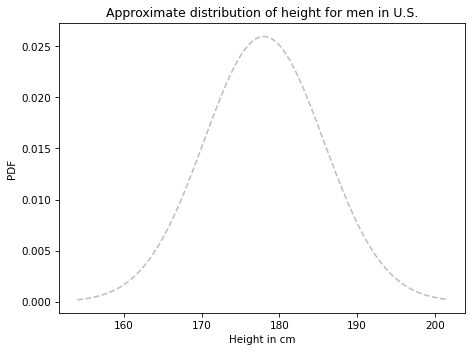
Here’s what it looks like.
from utils import decorate

prior.plot(style='--', color='C5')

decorate(xlabel='Height in cm',
         ylabel='PDF',
         title='Approximate distribution of height for men in U.S.')
This distribution represents what we believe about the heights of
A and
B before we take into account the data that
A is taller.
Section 11.3 Joint Distribution
The next step is to construct a distribution that represents the probability of every pair of heights, which is called a joint distribution. The elements of the joint distribution are
\begin{equation*}
P(A_x~\mathrm{and}~B_y)
\end{equation*}
which is the probability that
A is
\(x\) cm tall and
B is
\(y\) cm tall, for all values of
\(x\) and
\(y\text{.}\)
At this point all we know about
A and
B is that they are male residents of the U.S., so their heights are independent; that is, knowing the height of
A provides no additional information about the height of
B.
In that case, we can compute the joint probabilities like this:
\begin{equation*}
P(A_x~\mathrm{and}~B_y) = P(A_x)~P(B_y)
\end{equation*}
Each joint probability is the product of one element from the distribution of
x and one element from the distribution of
y.
So if we have
Pmf objects that represent the distribution of height for
A and
B, we can compute the joint distribution by computing the outer product of the probabilities in each
Pmf.
The following function takes two
Pmf objects and returns a
DataFrame that represents the joint distribution.
def make_joint(pmf1, pmf2):
    """Compute the outer product of two Pmfs."""
    X, Y = np.meshgrid(pmf1, pmf2)
    return pd.DataFrame(X * Y, columns=pmf1.qs, index=pmf2.qs)
The column names in the result are the quantities from
pmf1; the row labels are the quantities from
pmf2.
In this example, the prior distributions for
A and
B are the same, so we can compute the joint prior distribution like this:
joint = make_joint(prior, prior)
joint.shape
(96, 96)
The result is a
DataFrame with possible heights of
A along the columns, heights of
B along the rows, and the joint probabilities as elements.
If the prior is normalized, the joint prior is also normalized.
1.0
To add up all of the elements, we convert the
DataFrame to a NumPy array before calling
sum. Otherwise,
DataFrame.sum would compute the sums of the columns and return a
Series.
series = joint.sum()
series.shape
(96,)
Section 11.4 Visualizing the Joint Distribution
The following function uses
pcolormesh to plot the joint distribution.
import matplotlib.pyplot as plt

def plot_joint(joint, cmap='Blues'):
    """Plot a joint distribution with a color mesh."""
    vmax = joint.to_numpy().max() * 1.1
    plt.pcolormesh(joint.columns, joint.index, joint,
                   cmap=cmap,
                   vmax=vmax,
                   shading='nearest')
    plt.colorbar()

    decorate(xlabel='A height in cm',
             ylabel='B height in cm')
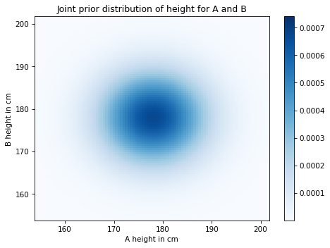
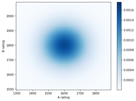
Here’s what the joint prior distribution looks like.
plot_joint(joint)
decorate(title='Joint prior distribution of height for A and B')
As you might expect, the probability is highest (darkest) near the mean and drops off farther from the mean.
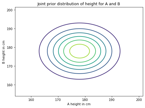
Another way to visualize the joint distribution is a contour plot.
def plot_contour(joint):
    """Plot a joint distribution with a contour."""
    plt.contour(joint.columns, joint.index, joint,
                linewidths=2)
    decorate(xlabel='A height in cm',
             ylabel='B height in cm')
plot_contour(joint)
decorate(title='Joint prior distribution of height for A and B')
Each line represents a level of equal probability.
Section 11.5 Likelihood
Now that we have a joint prior distribution, we can update it with the data, which is that
A is taller than
B.
Each element in the joint distribution represents a hypothesis about the heights of
A and
B. To compute the likelihood of every pair of quantities, we can extract the column names and row labels from the prior, like this:
x = joint.columns
y = joint.index
And use them to compute a mesh grid.
X contains copies of the quantities in
x, which are possible heights for
A.
Y contains copies of the quantities in
y, which are possible heights for
B.
If we compare
X and
Y, the result is a Boolean array:
A_taller = (X > Y)
A_taller.dtype
dtype('bool')
To compute likelihoods, I’ll use
np.where to make an array with
1 where
A_taller is
True and 0 elsewhere.
a = np.where(A_taller, 1, 0)
To visualize this array of likelihoods, I’ll put in a
DataFrame with the values of
x as column names and the values of
y as row labels.
likelihood = pd.DataFrame(a, index=x, columns=y)
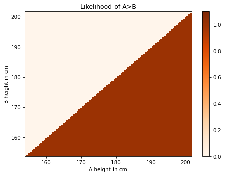
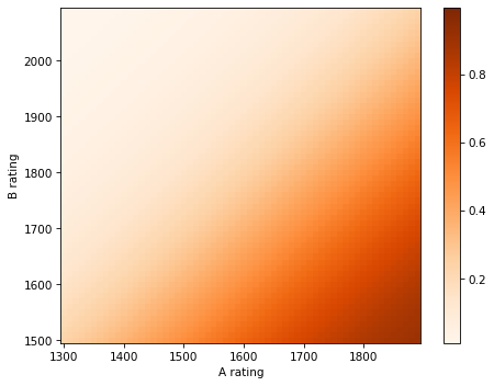
Here’s what it looks like:
plot_joint(likelihood, cmap='Oranges')
decorate(title='Likelihood of A>B')
The likelihood of the data is 1 where
X > Y and 0 elsewhere.
Section 11.7 Marginal Distributions
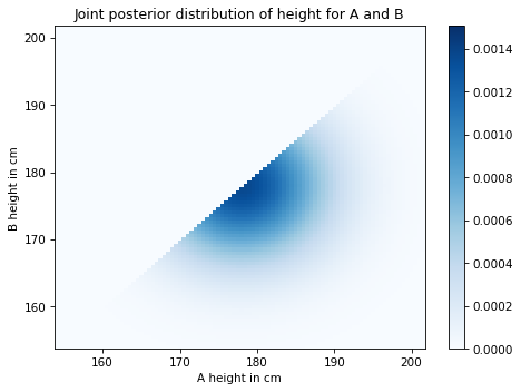
The joint posterior distribution represents what we believe about the heights of
A and
B given the prior distributions and the information that
A is taller.
From this joint distribution, we can compute the posterior distributions for
A and
B. To see how, let’s start with a simpler problem.
Suppose we want to know the probability that
A is 180 cm tall. We can select the column from the joint distribution where
x=180.
column = posterior[180]
column.head()
154.0    0.000010
154.5    0.000013
155.0    0.000015
155.5    0.000019
156.0    0.000022
Name: 180.0, dtype: float64
This column contains posterior probabilities for all cases where
x=180; if we add them up, we get the total probability that
A is 180 cm tall.
0.03017221271570807
Now, to get the posterior distribution of height for
A, we can add up all of the columns, like this:
column_sums = posterior.sum(axis=0)
column_sums.head()
154.0    0.000000e+00
154.5    1.012260e-07
155.0    2.736152e-07
155.5    5.532519e-07
156.0    9.915650e-07
dtype: float64
The argument
axis=0 means we want to add up the columns.
The result is a
Series that contains every possible height for
A and its probability. In other words, it is the distribution of heights for
A.
We can put it in a
Pmf like this:
marginal_A = Pmf(column_sums)
When we extract the distribution of a single variable from a joint distribution, the result is called a
marginal distribution. The name comes from a common visualization that shows the joint distribution in the middle and the marginal distributions in the margins.
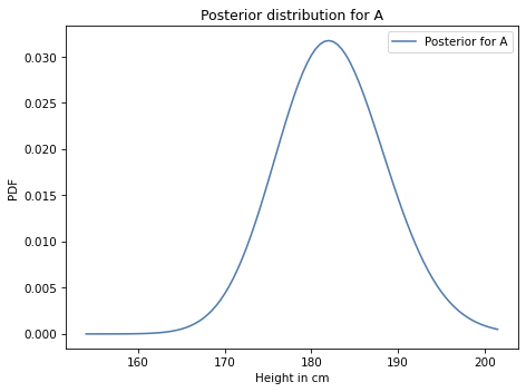
Here’s what the marginal distribution for
A looks like:
marginal_A.plot(label='Posterior for A')

decorate(xlabel='Height in cm',
         ylabel='PDF',
         title='Posterior distribution for A')
Similarly, we can get the posterior distribution of height for
B by adding up the rows and putting the result in a
Pmf.
row_sums = posterior.sum(axis=1)
marginal_B = Pmf(row_sums)
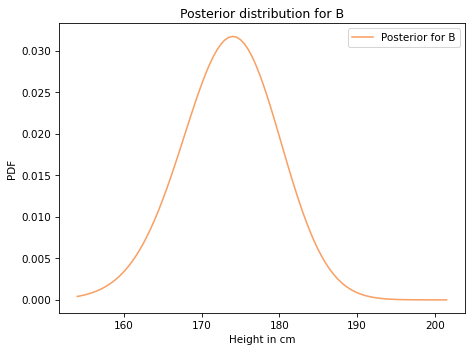
Here’s what it looks like.
marginal_B.plot(label='Posterior for B', color='C1')

decorate(xlabel='Height in cm',
         ylabel='PDF',
         title='Posterior distribution for B')
Let’s put the code from this section in a function:
def marginal(joint, axis):
    """Compute a marginal distribution."""
    return Pmf(joint.sum(axis=axis))
marginal takes as parameters a joint distribution and an axis number:
-
If
axis=0, it returns the marginal of the first variable (the one on the x-axis);
-
If
axis=1, it returns the marginal of the second variable (the one on the y-axis).
So we can compute both marginals like this:
marginal_A = marginal(posterior, axis=0)
marginal_B = marginal(posterior, axis=1)
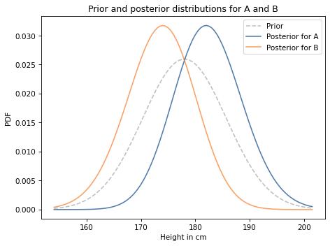
Here’s what they look like, along with the prior.
prior.plot(style='--', label='Prior', color='C5')
marginal_A.plot(label='Posterior for A')
marginal_B.plot(label='Posterior for B')

decorate(xlabel='Height in cm',
         ylabel='PDF',
         title='Prior and posterior distributions for A and B')
As you might expect, the posterior distribution for
A is shifted to the right and the posterior distribution for
B is shifted to the left.
We can summarize the results by computing the posterior means:
177.99516026921506
print(marginal_A.mean(), marginal_B.mean())
182.3872812342168 173.6028600023339
Based on the observation that
A is taller than
B, we are inclined to believe that
A is a little taller than average, and
B is a little shorter.
Notice that the posterior distributions are a little narrower than the prior. We can quantify that by computing their standard deviations.
7.624924796641578
print(marginal_A.std(), marginal_B.std())
6.270461177645469 6.280513548175111
The standard deviations of the posterior distributions are a little smaller, which means we are more certain about the heights of
A and
B after we compare them.
Section 11.8 Conditional Posteriors
Now suppose we measure
A and find that he is 170 cm tall. What does that tell us about
B?
In the joint distribution, each column corresponds a possible height for
A. We can select the column that corresponds to height 170 cm like this:
column_170 = posterior[170]
The result is a
Series that represents possible heights for
B and their relative likelihoods. These likelihoods are not normalized, but we can normalize them like this:
cond_B = Pmf(column_170)
cond_B.normalize()
0.004358061205454471
Making a
Pmf copies the data by default, so we can normalize
cond_B without affecting
column_170 or
posterior. The result is the conditional distribution of height for
B given that
A is 170 cm tall.
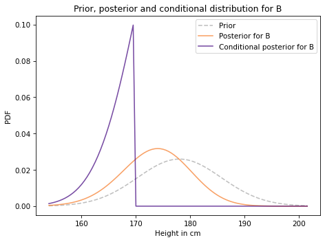
Here’s what it looks like:
prior.plot(style='--', label='Prior', color='C5')
marginal_B.plot(label='Posterior for B', color='C1')
cond_B.plot(label='Conditional posterior for B',
            color='C4')

decorate(xlabel='Height in cm',
         ylabel='PDF',
         title='Prior, posterior and conditional distribution for B')
The conditional posterior distribution is cut off at 170 cm, because we have established that
B is shorter than
A, and
A is 170 cm.