2.
This exercise is inspired by a true story. In 2001 I created
Green Tea Press to publish my books, starting with
Think Python. I ordered 100 copies from a short run printer and made the book available for sale through a distributor.
After the first week, the distributor reported that 12 copies were sold. Based that report, I thought I would run out of copies in about 8 weeks, so I got ready to order more. My printer offered me a discount if I ordered more than 1000 copies, so I went a little crazy and ordered 2000.
A few days later, my mother called to tell me that her
copies of the book had arrived. Surprised, I asked how many. She said ten.
It turned out I had sold only two books to non-relatives. And it took a lot longer than I expected to sell 2000 copies.
The details of this story are unique, but the general problem is something almost every retailer has to figure out. Based on past sales, how do you predict future sales? And based on those predictions, how do you decide how much to order and when?
Often the cost of a bad decision is complicated. If you place a lot of small orders rather than one big one, your costs are likely to be higher. If you run out of inventory, you might lose customers. And if you order too much, you have to pay the various costs of holding inventory.
So, let’s solve a version of the problem I faced. It will take some work to set up the problem; the details are in the notebook for this chapter.
Suppose you start selling books online. During the first week you sell 10 copies (and let’s assume that none of the customers are your mother). During the second week you sell 9 copies.
Assuming that the arrival of orders is a Poisson process, we can think of the weekly orders as samples from a Poisson distribution with an unknown rate. We can use orders from past weeks to estimate the parameter of this distribution, generate a predictive distribution for future weeks, and compute the order size that maximized expected profit.
-
Suppose the cost of printing the book is $5 per copy,
-
But if you order 100 or more, it’s $4.50 per copy.
-
For every book you sell, you get $10.
-
But if you run out of books before the end of 8 weeks, you lose $50 in future sales for every week you are out of stock.
-
If you have books left over at the end of 8 weeks, you lose $2 in inventory costs per extra book.
For example, suppose you get orders for 10 books per week, every week. If you order 60 books,
-
-
You sell all 60 books, so you make $600.
-
But the book is out of stock for two weeks, so you lose $100 in future sales.
In total, your profit is $200.
-
-
You sell 80 books, so you make $800.
-
But you have 20 books left over at the end, so you lose $40.
In total, your profit is $310.
Combining these costs with your predictive distribution, how many books should you order to maximize your expected profit?
To get you started, the following functions compute profits and costs according to the specification of the problem:
def print_cost(printed):
    """Compute print costs.

    printed: integer number printed
    """
    if printed < 100:
        return printed * 5
    else:
        return printed * 4.5
def total_income(printed, orders):
    """Compute income.

    printed: integer number printed
    orders: sequence of integer number of books ordered
    """
    sold = min(printed, np.sum(orders))
    return sold * 10
def inventory_cost(printed, orders):
    """Compute inventory costs.

    printed: integer number printed
    orders: sequence of integer number of books ordered
    """
    excess = printed - np.sum(orders)
    if excess > 0:
        return excess * 2
    else:
        return 0
def out_of_stock_cost(printed, orders):
    """Compute out of stock costs.

    printed: integer number printed
    orders: sequence of integer number of books ordered
    """
    weeks = len(orders)
    total_orders = np.cumsum(orders)
    for i, total in enumerate(total_orders):
        if total > printed:
            return (weeks-i) * 50
    return 0
def compute_profit(printed, orders):
    """Compute profit.

    printed: integer number printed
    orders: sequence of integer number of books ordered
    """
    return (total_income(printed, orders) -
            print_cost(printed)-
            out_of_stock_cost(printed, orders) -
            inventory_cost(printed, orders))
To test these functions, suppose we get exactly 10 orders per week for eight weeks:
always_10 = [10] * 8
always_10
[10, 10, 10, 10, 10, 10, 10, 10]
If you print 60 books, your net profit is $200, as in the example.
compute_profit(60, always_10)
200
If you print 100 books, your net profit is $310.
compute_profit(100, always_10)
310.0
Of course, in the context of the problem you don’t know how many books will be ordered in any given week. You don’t even know the average rate of orders. However, given the data and some assumptions about the prior, you can compute the distribution of the rate of orders.
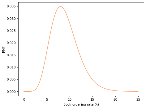
You’ll have a chance to do that, but to demonstrate the decision analysis part of the problem, I’ll start with the arbitrary assumption that order rates come from a gamma distribution with mean 9.
Here’s a
Pmf that represents this distribution.
from scipy.stats import gamma

alpha = 9
qs = np.linspace(0, 25, 101)
ps = gamma.pdf(qs, alpha)
pmf = Pmf(ps, qs)
pmf.normalize()
pmf.mean()
8.998788382371902
And here’s what it looks like:
pmf.plot(color='C1')
decorate(xlabel=r'Book ordering rate ($\lambda$)',
        ylabel='PMF')
Now, we could generate a predictive distribution for the number of books ordered in a given week, but in this example we have to deal with a complicated cost function. In particular,
out_of_stock_cost depends on the sequence of orders.
So, rather than generate a predictive distribution, I suggest we run simulations. I’ll demonstrate the steps.
First, from our hypothetical distribution of rates, we can draw a random sample of 1000 values.
rates = pmf.choice(1000)
np.mean(rates)
9.0135
For each possible rate, we can generate a sequence of 8 orders.
np.random.seed(17)
order_array = np.random.poisson(rates, size=(8, 1000)).transpose()
order_array[:5, :]
array([[10, 18, 14, 12, 15, 11, 21,  9],
       [ 6,  7,  5, 12, 15,  3,  3,  8],
       [ 6, 11, 11,  6,  6,  3,  7, 11],
       [12, 10,  9, 12, 16,  7, 11,  8],
       [11, 11,  8, 11, 10, 19, 24, 15]])
Each row of this array is a hypothetical sequence of orders based on a different hypothetical order rate.
Now, if you tell me how many books you printed, I can compute your expected profits, averaged over these 1000 possible sequences.
def compute_expected_profits(printed, order_array):
    """Compute profits averaged over a sample of orders.

    printed: number printed
    order_array: one row per sample, one column per week
    """
    profits = [compute_profit(printed, orders)
               for orders in order_array]
    return np.mean(profits)
For example, here are the expected profits if you order 70, 80, or 90 books.
compute_expected_profits(70, order_array)
190.474
compute_expected_profits(80, order_array)
190.774
compute_expected_profits(90, order_array)
164.484
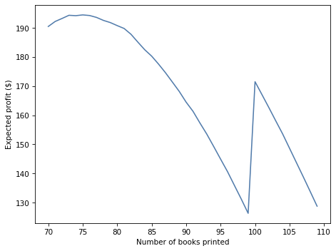
Now, let’s sweep through a range of values and compute expected profits as a function of the number of books you print.
printed_array = np.arange(70, 110)
t = [compute_expected_profits(printed, order_array)
                    for printed in printed_array]
expected_profits = pd.Series(t, printed_array)
expected_profits.plot(label='')

decorate(xlabel='Number of books printed',
         ylabel='Expected profit ($)')
Here is the optimal order and the expected profit.
expected_profits.idxmax(), expected_profits.max()
(75, 194.444)
Now it’s your turn. Choose a prior that you think is reasonable, update it with the data you are given, and then use the posterior distribution to do the analysis demonstrated in the notebook.
Solution.
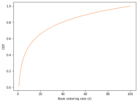
Choose a prior distribution (log-uniform from 1 to 100 books per week):
# For a prior I chose a log-uniform distribution;
# that is, a distribution that is uniform in log-space
# from 1 to 100 books per week.

qs = np.logspace(0, 2, 101)
prior = Pmf(1, qs)
prior.normalize()
101
# Here's the CDF of the prior

prior.make_cdf().plot(color='C1')
decorate(xlabel=r'Book ordering rate ($\lambda$)',
         ylabel='CDF')
# Here's a function that updates the distribution of lambda
# based on one week of orders

from scipy.stats import poisson

def update_book(pmf, data):
    """Update book ordering rate.

    pmf: Pmf of book ordering rates
    data: observed number of orders in one week
    """
    k = data
    lams = pmf.index
    likelihood = poisson.pmf(k, lams)
    pmf *= likelihood
    pmf.normalize()
# Here's the update after week 1.

posterior1 = prior.copy()
update_book(posterior1, 10)
# And the update after week 2.

posterior2 = posterior1.copy()
update_book(posterior2, 9)
prior.mean(), posterior1.mean(), posterior2.mean()
(21.78849107458653, 10.000000817984526, 9.500000000003652)
# Now we can generate a sample of 1000 values from the posterior

rates = posterior2.choice(1000)
np.mean(rates)
9.568378334655758
# And we can generate a sequence of 8 weeks for each value

order_array = np.random.poisson(rates, size=(8, 1000)).transpose()
order_array[:5, :]
array([[ 9,  6,  6,  6,  9,  8, 11,  9],
       [ 4,  5,  3,  1,  6,  3,  4,  4],
       [ 5,  7,  7, 10,  4,  7, 12, 10],
       [ 4,  4, 10,  6, 10, 19,  9, 10],
       [ 9, 11, 13,  8,  8, 13, 18,  3]])
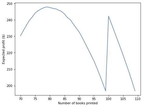
# Here are the expected profits for each possible order

printed_array = np.arange(70, 110)
t = [compute_expected_profits(printed, order_array)
                    for printed in printed_array]
expected_profits = pd.Series(t, printed_array)
# And here's what they look like.

expected_profits.plot(label='')

decorate(xlabel='Number of books printed',
         ylabel='Expected profit ($)')
# Here's the optimal order.

expected_profits.idxmax()
79