Section 15.1 The Grizzly Bear Problem
In 1996 and 1997 researchers deployed bear traps in locations in British Columbia and Alberta, Canada, in an effort to estimate the population of grizzly bears. They describe the experiment in
this article.
The "trap" consists of a lure and several strands of barbed wire intended to capture samples of hair from bears that visit the lure. Using the hair samples, the researchers use DNA analysis to identify individual bears.
During the first session, the researchers deployed traps at 76 sites. Returning 10 days later, they obtained 1043 hair samples and identified 23 different bears. During a second 10-day session they obtained 1191 samples from 19 different bears, where 4 of the 19 were from bears they had identified in the first batch.
To estimate the population of bears from this data, we need a model for the probability that each bear will be observed during each session. As a starting place, we’ll make the simplest assumption, that every bear in the population has the same (unknown) probability of being sampled during each session.
With these assumptions we can compute the probability of the data for a range of possible populations.
As an example, let’s suppose that the actual population of bears is 100.
After the first session, 23 of the 100 bears have been identified. During the second session, if we choose 19 bears at random, what is the probability that 4 of them were previously identified?
-
\(N\text{:}\) actual population size, 100.
-
\(K\text{:}\) number of bears identified in the first session, 23.
-
\(n\text{:}\) number of bears observed in the second session, 19 in the example.
-
\(k\text{:}\) number of bears in the second session that were previously identified, 4.
For given values of
\(N\text{,}\) \(K\text{,}\) and
\(n\text{,}\) the probability of finding
\(k\) previously-identified bears is given by the
hypergeometric distribution:
\begin{equation*}
\binom{K}{k} \binom{N-K}{n-k}/ \binom{N}{n}
\end{equation*}
where the
binomial coefficient,
\(\binom{K}{k}\text{,}\) is the number of subsets of size
\(k\) we can choose from a population of size
\(K\text{.}\)
To understand why, consider:
-
The denominator,
\(\binom{N}{n}\text{,}\) is the number of subsets of
\(n\) we could choose from a population of
\(N\) bears.
-
The numerator is the number of subsets that contain
\(k\) bears from the previously identified
\(K\) and
\(n-k\) from the previously unseen
\(N-K\text{.}\)
SciPy provides
hypergeom, which we can use to compute this probability for a range of values of
\(k\text{.}\)
import numpy as np
from scipy.stats import hypergeom

N = 100
K = 23
n = 19

ks = np.arange(12)
ps = hypergeom(N, K, n).pmf(ks)
The result is the distribution of
\(k\) with given parameters
\(N\text{,}\) \(K\text{,}\) and
\(n\text{.}\) Here’s what it looks like.
import matplotlib.pyplot as plt
from utils import decorate

plt.bar(ks, ps)

decorate(xlabel='Number of bears observed twice',
         ylabel='PMF',
         title='Hypergeometric distribution of k (known population 100)')
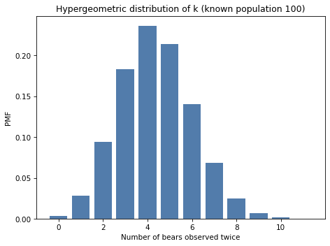
The most likely value of
\(k\) is 4, which is the value actually observed in the experiment. That suggests that
\(N=100\) is a reasonable estimate of the population, given this data.
We’ve computed the distribution of
\(k\) given
\(N\text{,}\) \(K\text{,}\) and
\(n\text{.}\) Now let’s go the other way: given
\(K\text{,}\) \(n\text{,}\) and
\(k\text{,}\) how can we estimate the total population,
\(N\text{?}\)
Section 15.2 The Update
As a starting place, let’s suppose that, prior to this study, an expert estimates that the local bear population is between 50 and 500, and equally likely to be any value in that range.
I’ll use
make_uniform to make a uniform distribution of integers in this range.
import numpy as np
from utils import make_uniform

qs = np.arange(50, 501)
prior_N = make_uniform(qs, name='N')
prior_N.shape
(451,)
To compute the likelihood of the data, we can use
hypergeom with constants
K and
n, and a range of values of
N.
Ns = prior_N.qs
K = 23
n = 19
k = 4

likelihood = hypergeom(Ns, K, n).pmf(k)
We can compute the posterior in the usual way.
posterior_N = prior_N * likelihood
posterior_N.normalize()
0.07755224277106798
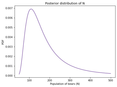
And here’s what it looks like.
posterior_N.plot(color='C4')

decorate(xlabel='Population of bears (N)',
         ylabel='PDF',
         title='Posterior distribution of N')
The most likely value is 109.
109
But the distribution is skewed to the right, so the posterior mean is substantially higher.
173.79880627085805
And the credible interval is quite wide.
posterior_N.credible_interval(0.9)
array([ 77., 363.])
This solution is relatively simple, but it turns out we can do a little better if we model the unknown probability of observing a bear explicitly.
Section 15.3 Two-Parameter Model
Next we’ll try a model with two parameters: the number of bears,
N, and the probability of observing a bear,
p.
We’ll assume that the probability is the same in both rounds, which is probably reasonable in this case because it is the same kind of trap in the same place.
We’ll also assume that the probabilities are independent; that is, the probability a bear is observed in the second round does not depend on whether it was observed in the first round. This assumption might be less reasonable, but for now it is a necessary simplification.
Here are the counts again:
For this model, I’ll express the data in a notation that will make it easier to generalize to more than two rounds:
-
k10 is the number of bears observed in the first round but not the second,
-
k01 is the number of bears observed in the second round but not the first, and
-
k11 is the number of bears observed in both rounds.
k10 = 23 - 4
k01 = 19 - 4
k11 = 4
Suppose we know the actual values of
N and
p. We can use them to compute the likelihood of this data.
For example, suppose we know that
N=100 and
p=0.2. We can use
N to compute
k00, which is the number of unobserved bears.
N = 100

observed = k01 + k10 + k11
k00 = N - observed
k00
62
For the update, it will be convenient to store the data as a list that represents the number of bears in each category.
x = [k00, k01, k10, k11]
x
[62, 15, 19, 4]
Now, if we know
p=0.2, we can compute the probability a bear falls in each category. For example, the probability of being observed in both rounds is
p*p, and the probability of being unobserved in both rounds is
q*q (where
q=1-p).
p = 0.2
q = 1-p
y = [q*q, q*p, p*q, p*p]
y
[0.6400000000000001,
 0.16000000000000003,
 0.16000000000000003,
 0.04000000000000001]
\begin{equation*}
\frac{N!}{\prod x_i!} \prod y_i^{x_i}
\end{equation*}
where
\(N\) is actual population,
\(x\) is a sequence with the counts in each category, and
\(y\) is a sequence of probabilities for each category.
SciPy provides
multinomial, which provides
pmf, which computes this probability. Here is the probability of the data for these values of
N and
p.
from scipy.stats import multinomial

likelihood = multinomial.pmf(x, N, y)
likelihood
0.0016664011988507257
That’s the likelihood if we know
N and
p, but of course we don’t. So we’ll choose prior distributions for
N and
p, and use the likelihoods to update it.
Section 15.4 The Prior
We’ll use
prior_N again for the prior distribution of
N, and a uniform prior for the probability of observing a bear,
p:
qs = np.linspace(0, 0.99, num=100)
prior_p = make_uniform(qs, name='p')
We can make a joint distribution in the usual way.
from utils import make_joint

joint_prior = make_joint(prior_p, prior_N)
joint_prior.shape
(451, 100)
The result is a Pandas
DataFrame with values of
N down the rows and values of
p across the columns. However, for this problem it will be convenient to represent the prior distribution as a 1-D
Series rather than a 2-D
DataFrame. We can convert from one format to the other using
stack.
from empiricaldist import Pmf

joint_pmf = Pmf(joint_prior.stack())
joint_pmf.head(3)
           probs
N   p
50  0.00    0.000022
    0.01    0.000022
    0.02    0.000022
dtype: float64
empiricaldist.empiricaldist.Pmf
pandas.core.indexes.multi.MultiIndex
(45100,)
The result is a
Pmf whose index is a
MultiIndex. A
MultiIndex can have more than one column; in this example, the first column contains values of
N and the second column contains values of
p.
The
Pmf has one row (and one prior probability) for each possible pair of parameters
N and
p. So the total number of rows is the product of the lengths of
prior_N and
prior_p.
Now we have to compute the likelihood of the data for each pair of parameters.
Section 15.5 The Update
To allocate space for the likelihoods, it is convenient to make a copy of
joint_pmf:
likelihood = joint_pmf.copy()
As we loop through the pairs of parameters, we compute the likelihood of the data as in the previous section, and then store the result as an element of
likelihood.
observed = k01 + k10 + k11

for N, p in joint_pmf.index:
    k00 = N - observed
    x = [k00, k01, k10, k11]
    q = 1-p
    y = [q*q, q*p, p*q, p*p]
    likelihood[N, p] = multinomial.pmf(x, N, y)
Now we can compute the posterior in the usual way.
posterior_pmf = joint_pmf * likelihood
posterior_pmf.normalize()
2.9678796190279657e-05
We’ll use
plot_contour again to visualize the joint posterior distribution. But remember that the posterior distribution we just computed is represented as a
Pmf, which is a
Series, and
plot_contour expects a
DataFrame.
Since we used
stack to convert from a
DataFrame to a
Series, we can use
unstack to go the other way.
joint_posterior = posterior_pmf.unstack()
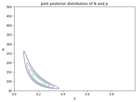
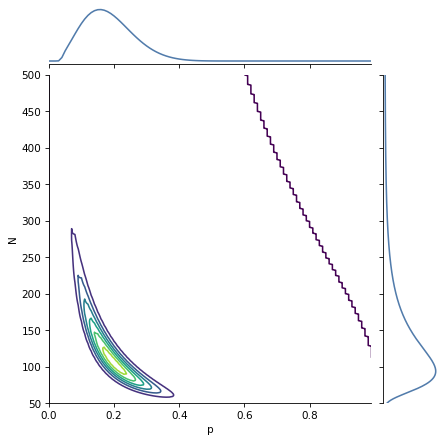
And here’s what the result looks like.
from utils import plot_contour

plot_contour(joint_posterior)

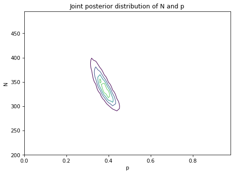
decorate(title='Joint posterior distribution of N and p')
The most likely values of
N are near 100, as in the previous model. The most likely values of
p are near 0.2.
The shape of this contour indicates that these parameters are correlated. If
p is near the low end of the range, the most likely values of
N are higher; if
p is near the high end of the range,
N is lower.
Now that we have a posterior
DataFrame, we can extract the marginal distributions in the usual way.
from utils import marginal

posterior2_p = marginal(joint_posterior, 0)
posterior2_N = marginal(joint_posterior, 1)
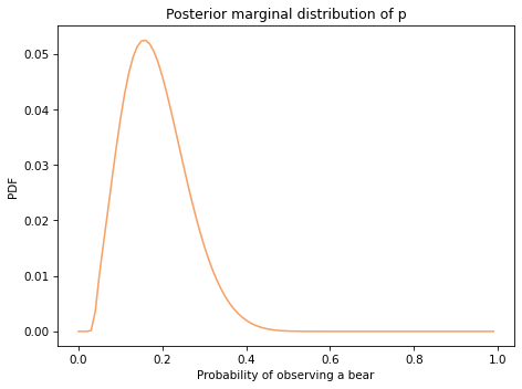
Here’s the posterior distribution for
p:
posterior2_p.plot(color='C1')

decorate(xlabel='Probability of observing a bear',
         ylabel='PDF',
         title='Posterior marginal distribution of p')
The most likely values are near 0.2.
Here’s the posterior distribution for
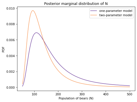
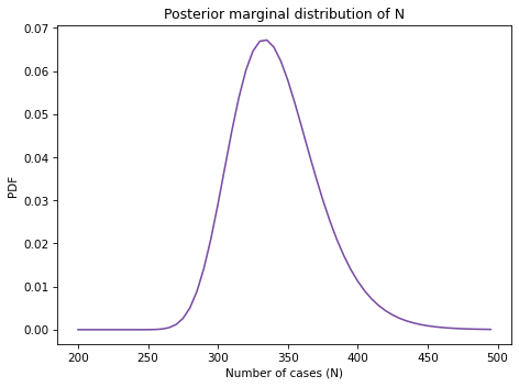
N based on the two-parameter model, along with the posterior we got using the one-parameter (hypergeometric) model.
posterior_N.plot(label='one-parameter model', color='C4')
posterior2_N.plot(label='two-parameter model', color='C1')

decorate(xlabel='Population of bears (N)',
         ylabel='PDF',
         title='Posterior marginal distribution of N')
With the two-parameter model, the mean is a little lower and the 90% credible interval is a little narrower.
print(posterior_N.mean(), posterior_N.credible_interval(0.9))
173.79880627085805 [ 77. 363.]
print(posterior2_N.mean(), posterior2_N.credible_interval(0.9))
138.750521364726 [ 68. 277.]
The two-parameter model yields a narrower posterior distribution for
N, compared to the one-parameter model, because it takes advantage of an additional source of information: the consistency of the two observations.
To see how this helps, consider a scenario where
N is relatively low, like 138 (the posterior mean of the two-parameter model).
Given that we saw 23 bears during the first trial and 19 during the second, we can estimate the corresponding value of
p.
mean = (23 + 19) / 2
p = mean/N1
p
0.15217391304347827
With these parameters, how much variability do you expect in the number of bears from one trial to the next? We can quantify that by computing the standard deviation of the binomial distribution with these parameters.
from scipy.stats import binom

binom(N1, p).std()
4.219519857292647
Now let’s consider a second scenario where
N is 173, the posterior mean of the one-parameter model. The corresponding value of
p is lower.
0.12138728323699421
In this scenario, the variation we expect to see from one trial to the next is higher.
4.2954472470306415
So if the number of bears we observe is the same in both trials, that would be evidence for lower values of
N, where we expect more consistency. If the number of bears is substantially different between the two trials, that would be evidence for higher values of
N.
In the actual data, the difference between the two trials is low, which is why the posterior mean of the two-parameter model is lower. The two-parameter model takes advantage of additional information, which is why the credible interval is narrower.
Section 15.7 The Lincoln Index Problem
In an excellent blog post, John D. Cook wrote about the Lincoln index, which is a way to estimate the number of errors in a document (or program) by comparing results from two independent testers. Here’s his presentation of the problem:
Suppose you have a tester who finds 20 bugs in your program. You want to estimate how many bugs are really in the program. You know there are at least 20 bugs, and if you have supreme confidence in your tester, you may suppose there are around 20 bugs. But maybe your tester isn’t very good. Maybe there are hundreds of bugs. How can you have any idea how many bugs there are? There’s no way to know with one tester. But if you have two testers, you can get a good idea, even if you don’t know how skilled the testers are.
Suppose the first tester finds 20 bugs, the second finds 15, and they find 3 in common; how can we estimate the number of bugs?
This problem is similar to the Grizzly Bear problem, so I’ll represent the data in the same way.
k10 = 20 - 3
k01 = 15 - 3
k11 = 3
But in this case it is probably not reasonable to assume that the testers have the same probability of finding a bug. So I’ll define two parameters,
p0 for the probability that the first tester finds a bug, and
p1 for the probability that the second tester finds a bug.
I will continue to assume that the probabilities are independent, which is like assuming that all bugs are equally easy to find. That might not be a good assumption, but let’s stick with it for now.
As an example, suppose we know that the probabilities are 0.2 and 0.15.
We can compute the array of probabilities,
y, like this:
def compute_probs(p0, p1):
    """Computes the probability for each of 4 categories."""
    q0 = 1-p0
    q1 = 1-p1
    return [q0*q1, q0*p1, p0*q1, p0*p1]
y = compute_probs(p0, p1)
y
[0.68, 0.12, 0.17, 0.03]
With these probabilities, there is a 68% chance that neither tester finds the bug and a 3% chance that both do.
Pretending that these probabilities are known, we can compute the posterior distribution for
N. Here’s a prior distribution that’s uniform from 32 to 350 bugs.
qs = np.arange(32, 350, step=5)
prior_N = make_uniform(qs, name='N')
prior_N.head(3)
        probs
N
32    0.015625
37    0.015625
42    0.015625
dtype: float64
I’ll put the data in an array, with 0 as a place-keeper for the unknown value
k00.
data = np.array([0, k01, k10, k11])
And here are the likelihoods for each value of
N, with
ps as a constant.
likelihood = prior_N.copy()
observed = data.sum()
x = data.copy()

for N in prior_N.qs:
    x[0] = N - observed
    likelihood[N] = multinomial.pmf(x, N, y)
We can compute the posterior in the usual way.
posterior_N = prior_N * likelihood
posterior_N.normalize()
0.0003425201572557094
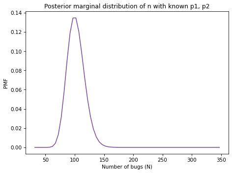
And here’s what it looks like.
posterior_N.plot(color='C4')

decorate(xlabel='Number of bugs (N)',
         ylabel='PMF',
         title='Posterior marginal distribution of N with known p0, p1')
print(posterior_N.mean(), posterior_N.credible_interval(0.9))
102.1249999999998 [ 77. 127.]
With the assumption that
p0 and
p1 are known to be
0.2 and
0.15, the posterior mean is 102 with 90% credible interval (77, 127). But this result is based on the assumption that we know the probabilities, and we don’t.
Section 15.8 Three-Parameter Model
What we need is a model with three parameters:
N,
p0, and
p1. We’ll use
prior_N again for the prior distribution of
N, and here are the priors for
p0 and
p1:
qs = np.linspace(0, 1, num=51)
prior_p0 = make_uniform(qs, name='p0')
prior_p1 = make_uniform(qs, name='p1')
Now we have to assemble them into a joint prior with three dimensions. I’ll start by putting the first two into a
DataFrame.
joint2 = make_joint(prior_p0, prior_N)
joint2.shape
(64, 51)
Now I’ll stack them, as in the previous example, and put the result in a
Pmf.
joint2_pmf = Pmf(joint2.stack())
joint2_pmf.head(3)
              probs
N   p0
32  0.00    0.000306
    0.02    0.000306
    0.04    0.000306
dtype: float64
We can use
make_joint again to add in the third parameter.
joint3 = make_joint(prior_p1, joint2_pmf)
joint3.shape
(3264, 51)
The result is a
DataFrame with values of
N and
p0 in a
MultiIndex that goes down the rows and values of
p1 in an index that goes across the columns.
p1           0.00      0.02      0.04      0.06      0.08      0.10      0.12  \
N  p0
32 0.00  0.000006  0.000006  0.000006  0.000006  0.000006  0.000006  0.000006
   0.02  0.000006  0.000006  0.000006  0.000006  0.000006  0.000006  0.000006
   0.04  0.000006  0.000006  0.000006  0.000006  0.000006  0.000006  0.000006

p1           0.14      0.16      0.18  ...      0.82      0.84      0.86  \
N  p0                                  ...
32 0.00  0.000006  0.000006  0.000006  ...  0.000006  0.000006  0.000006
   0.02  0.000006  0.000006  0.000006  ...  0.000006  0.000006  0.000006
   0.04  0.000006  0.000006  0.000006  ...  0.000006  0.000006  0.000006

p1           0.88      0.90      0.92      0.94      0.96      0.98      1.00
N  p0
32 0.00  0.000006  0.000006  0.000006  0.000006  0.000006  0.000006  0.000006
   0.02  0.000006  0.000006  0.000006  0.000006  0.000006  0.000006  0.000006
   0.04  0.000006  0.000006  0.000006  0.000006  0.000006  0.000006  0.000006

[3 rows x 51 columns]
Now I’ll apply
stack again:
joint3_pmf = Pmf(joint3.stack())
joint3_pmf.head(3)
                   probs
N   p0   p1
32  0.0  0.00    0.000006
         0.02    0.000006
         0.04    0.000006
dtype: float64
The result is a
Pmf with a three-column
MultiIndex containing all possible triplets of parameters.
The number of rows is the product of the number of values in all three priors, which is almost 170,000.
(166464,)
That’s still small enough to be practical, but it will take longer to compute the likelihoods than in the previous examples.
Here’s the loop that computes the likelihoods; it’s similar to the one in the previous section:
likelihood = joint3_pmf.copy()
observed = data.sum()
x = data.copy()

for N, p0, p1 in joint3_pmf.index:
    x[0] = N - observed
    y = compute_probs(p0, p1)
    likelihood[N, p0, p1] = multinomial.pmf(x, N, y)
We can compute the posterior in the usual way.
posterior_pmf = joint3_pmf * likelihood
posterior_pmf.normalize()
8.941088283758206e-06
Now, to extract the marginal distributions, we could unstack the joint posterior as we did in the previous section. But
Pmf provides a version of
marginal that works with a
Pmf rather than a
DataFrame. Here’s how we use it to get the posterior distribution for
N.
posterior_N = posterior_pmf.marginal(0)
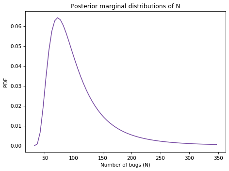
And here’s what it looks like.
posterior_N.plot(color='C4')

decorate(xlabel='Number of bugs (N)',
         ylabel='PDF',
         title='Posterior marginal distributions of N')
105.76561732196238
The posterior mean is 105 bugs, which suggests that there are still many bugs the testers have not found.
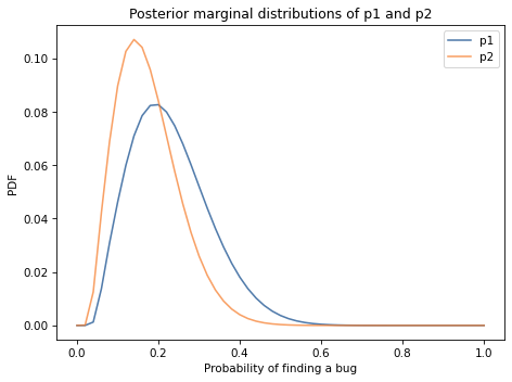
Here are the posteriors for
p0 and
p1.
posterior_p1 = posterior_pmf.marginal(1)
posterior_p2 = posterior_pmf.marginal(2)

posterior_p1.plot(label='p1')
posterior_p2.plot(label='p2')

decorate(xlabel='Probability of finding a bug',
         ylabel='PDF',
         title='Posterior marginal distributions of p1 and p2')
posterior_p1.mean(), posterior_p1.credible_interval(0.9)
(0.2297065971677734, array([0.1, 0.4]))
posterior_p2.mean(), posterior_p2.credible_interval(0.9)
(0.17501172155925765, array([0.06, 0.32]))
Comparing the posterior distributions, the tester who found more bugs probably has a higher probability of finding bugs. The posterior means are about 23% and 18%. But the distributions overlap, so we should not be too sure.
This is the first example we’ve seen with three parameters. As the number of parameters increases, the number of combinations increases quickly. The method we’ve been using so far, enumerating all possible combinations, becomes impractical if the number of parameters is more than 3 or 4.
However there are other methods that can handle models with many more parameters, as we’ll see in a later chapter on MCMC.