Section 6.1 Odds
One way to represent a probability is with a number between 0 and 1, but that’s not the only way. If you have ever bet on a football game or a horse race, you have probably encountered another representation of probability, called
odds.
You might have heard expressions like "the odds are three to one", but you might not know what that means. The
odds in favor of an event are the ratio of the probability it will occur to the probability that it will not.
The following function does this calculation.
def odds(p):
    return p / (1-p)
For example, if my team has a 75% chance of winning, the odds in their favor are three to one, because the chance of winning is three times the chance of losing.
3.0
You can write odds in decimal form, but it is also common to write them as a ratio of integers. So "three to one" is sometimes written
\(3:1\text{.}\)
When probabilities are low, it is more common to report the
odds against rather than the odds in favor. For example, if my horse has a 10% chance of winning, the odds in favor are
\(1:9\text{.}\)
0.11111111111111112
But in that case it would be more common I to say that the odds against are
\(9:1\text{.}\)
9.000000000000002
Given the odds in favor, in decimal form, you can convert to probability like this:
def prob(o):
    return o / (o+1)
For example, if the odds are
\(3/2\text{,}\) the corresponding probability is
\(3/5\text{:}\)
0.6
Or if you represent odds with a numerator and denominator, you can convert to probability like this:
def prob2(yes, no):
    return yes / (yes + no)
0.6
Probabilities and odds are different representations of the same information; given either one, you can compute the other. But some computations are easier when we work with odds, as we’ll see in the next section, and some computations are even easier with log odds, which we’ll see later.
Section 6.2 Bayes’s Rule
So far we have worked with Bayes’s theorem in the "probability form":
\begin{equation*}
P(H|D) = \frac{P(H)~P(D|H)}{P(D)}
\end{equation*}
Writing
\(\mathrm{odds}(A)\) for odds in favor of
\(A\text{,}\) we can express Bayes’s Theorem in "odds form":
\begin{equation*}
\mathrm{odds}(A|D) = \mathrm{odds}(A)~\frac{P(D|A)}{P(D|B)}
\end{equation*}
This is Bayes’s Rule, which says that the posterior odds are the prior odds times the likelihood ratio. Bayes’s Rule is convenient for computing a Bayesian update on paper or in your head. For example, let’s go back to the cookie problem:
Suppose there are two bowls of cookies. Bowl 1 contains 30 vanilla cookies and 10 chocolate cookies. Bowl 2 contains 20 of each. Now suppose you choose one of the bowls at random and, without looking, select a cookie at random. The cookie is vanilla. What is the probability that it came from Bowl 1?
The prior probability is 50%, so the prior odds are 1. The likelihood ratio is
\(\frac{3}{4} / \frac{1}{2}\text{,}\) or
\(3/2\text{.}\) So the posterior odds are
\(3/2\text{,}\) which corresponds to probability
\(3/5\text{.}\)
prior_odds = 1
likelihood_ratio = (3/4) / (1/2)
post_odds = prior_odds * likelihood_ratio
post_odds
1.5
post_prob = prob(post_odds)
post_prob
0.6
If we draw another cookie and it’s chocolate, we can do another update:
likelihood_ratio = (1/4) / (1/2)
post_odds *= likelihood_ratio
post_odds
0.75
And convert back to probability.
post_prob = prob(post_odds)
post_prob
0.42857142857142855
Section 6.3 Oliver’s Blood
Two people have left traces of their own blood at the scene of a crime. A suspect, Oliver, is tested and found to have type ‘O’ blood. The blood groups of the two traces are found to be of type ‘O’ (a common type in the local population, having frequency 60%) and of type ‘AB’ (a rare type, with frequency 1%). Do these data [the traces found at the scene] give evidence in favor of the proposition that Oliver was one of the people [who left blood at the scene]?
To answer this question, we need to think about what it means for data to give evidence in favor of (or against) a hypothesis. Intuitively, we might say that data favor a hypothesis if the hypothesis is more likely in light of the data than it was before.
In the cookie problem, the prior odds are 1, which corresponds to probability 50%. The posterior odds are
\(3/2\text{,}\) or probability 60%. So the vanilla cookie is evidence in favor of Bowl 1.
Bayes’s Rule provides a way to make this intuition more precise. Again
\begin{equation*}
\mathrm{odds}(A|D) = \mathrm{odds}(A)~\frac{P(D|A)}{P(D|B)}
\end{equation*}
Dividing through by
\(\mathrm{odds}(A)\text{,}\) we get:
\begin{equation*}
\frac{\mathrm{odds}(A|D)}{\mathrm{odds}(A)} = \frac{P(D|A)}{P(D|B)}
\end{equation*}
The term on the left is the ratio of the posterior and prior odds. The term on the right is the likelihood ratio, also called the
Bayes factor.
If the Bayes factor is greater than 1, that means that the data were more likely under
\(A\) than under
\(B\text{.}\) And that means that the odds are greater, in light of the data, than they were before.
If the Bayes factor is less than 1, that means the data were less likely under
\(A\) than under
\(B\text{,}\) so the odds in favor of
\(A\) go down.
Finally, if the Bayes factor is exactly 1, the data are equally likely under either hypothesis, so the odds do not change.
Let’s apply that to the problem at hand. If Oliver is one of the people who left blood at the crime scene, he accounts for the ‘O’ sample; in that case, the probability of the data is the probability that a random member of the population has type ‘AB’ blood, which is 1%.
If Oliver did not leave blood at the scene, we have two samples to account for. If we choose two random people from the population, what is the chance of finding one with type ‘O’ and one with type ‘AB’? Well, there are two ways it might happen:
-
The first person might have ‘O’ and the second ‘AB’,
-
Or the first person might have ‘AB’ and the second ‘O’.
The probability of either combination is
\((0.6) (0.01)\text{,}\) which is 0.6%, so the total probability is twice that, or 1.2%. So the data are a little more likely if Oliver is
not one of the people who left blood at the scene.
We can use these probabilities to compute the likelihood ratio:
like1 = 0.01
like2 = 2 * 0.6 * 0.01

likelihood_ratio = like1 / like2
likelihood_ratio
0.8333333333333334
Since the likelihood ratio is less than 1, the blood tests are evidence
against the hypothesis that Oliver left blood at the scence.
But it is weak evidence. For example, if the prior odds were 1 (that is, 50% probability), the posterior odds would be 0.83, which corresponds to a probability of 45%:
post_odds = 1 * like1 / like2
prob(post_odds)
0.45454545454545453
So this evidence doesn’t "move the needle" very much.
This example is a little contrived, but it demonstrates the counterintuitive result that data
consistent with a hypothesis are not necessarily
in favor of the hypothesis.
If this result still bothers you, this way of thinking might help: the data consist of a common event, type ‘O’ blood, and a rare event, type ‘AB’ blood. If Oliver accounts for the common event, that leaves the rare event unexplained. If Oliver doesn’t account for the ‘O’ blood, we have two chances to find someone in the population with ‘AB’ blood. And that factor of two makes the difference.
Checkpoint 6.3.1. Exercise.
Suppose that based on other evidence, you prior belief in Oliver’s guilt is 90%. How much would the blood evidence in this section change your beliefs? What if you initially thought there was only a 10% chance of his guilt?
Solution.
post_odds = odds(0.9) * like1 / like2
prob(post_odds)
0.8823529411764706
post_odds = odds(0.1) * like1 / like2
prob(post_odds)
0.0847457627118644
Section 6.4 Addends
The second half of this chapter is about distributions of sums and results of other operations. We’ll start with a forward problem, where we are given the inputs and compute the distribution of the output. Then we’ll work on inverse problems, where we are given the outputs and we compute the distribution of the inputs.
As a first example, suppose you roll two dice and add them up. What is the distribution of the sum? I’ll use the following function to create a
Pmf that represents the possible outcomes of a die:
import numpy as np
from empiricaldist import Pmf

def make_die(sides):
    outcomes = np.arange(1, sides+1)
    die = Pmf(1/sides, outcomes)
    return die
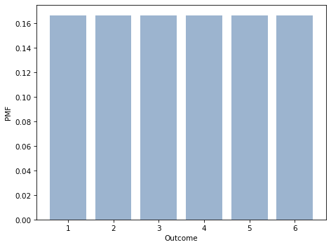
On a six-sided die, the outcomes are 1 through 6, all equally likely.
from utils import decorate

die.bar(alpha=0.4)
decorate(xlabel='Outcome',
         ylabel='PMF')
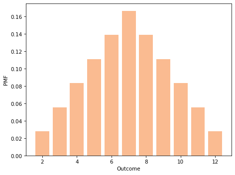
If we roll two dice and add them up, there are 11 possible outcomes, 2 through 12, but they are not equally likely. To compute the distribution of the sum, we have to enumerate the possible outcomes.
And that’s how this function works:
def add_dist(pmf1, pmf2):
    """Compute the distribution of a sum."""
    res = Pmf()
    for q1, p1 in pmf1.items():
        for q2, p2 in pmf2.items():
            q = q1 + q2
            p = p1 * p2
            res[q] = res(q) + p
    return res
The parameters are
Pmf objects representing distributions.
The loops iterate though the quantities and probabilities in the
Pmf objects. Each time through the loop
q gets the sum of a pair of quantities, and
p gets the probability of the pair. Because the same sum might appear more than once, we have to add up the total probability for each sum.
Notice a subtle element of this line:
\begin{equation*}
res[q] = res(q) + p
\end{equation*}
I use parentheses on the right side of the assignment, which returns 0 if
q does not appear yet in
res. I use brackets on the left side of the assignment to create or update an element in
res; using parentheses on the left side would not work.
Pmf provides
add_dist, which does the same thing. You can call it as a method, like this:
twice = die.add_dist(die)
Or as a function, like this:
twice = Pmf.add_dist(die, die)
And here’s what the result looks like:
from utils import decorate

def decorate_dice(title=''):
    decorate(xlabel='Outcome',
             ylabel='PMF',
             title=title)
twice = add_dist(die, die)
twice.bar(color='C1', alpha=0.5)
decorate_dice()
If we have a sequence of
Pmf objects that represent dice, we can compute the distribution of the sum like this:
def add_dist_seq(seq):
    """Compute Pmf of the sum of values from seq."""
    total = seq[0]
    for other in seq[1:]:
        total = total.add_dist(other)
    return total
As an example, we can make a list of three dice like this:
And we can compute the distribution of their sum like this.
thrice = add_dist_seq(dice)
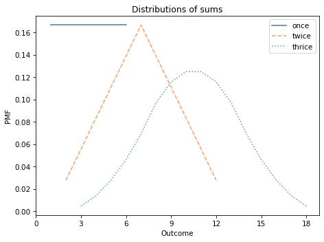
The following figure shows what these three distributions look like:
-
The distribution of a single die is uniform from 1 to 6.
-
The sum of two dice has a triangle distribution between 2 and 12.
-
The sum of three dice has a bell-shaped distribution between 3 and 18.
import matplotlib.pyplot as plt

die.plot(label='once')
twice.plot(label='twice', ls='--')
thrice.plot(label='thrice', ls=':')

plt.xticks([0,3,6,9,12,15,18])
decorate_dice(title='Distributions of sums')
As an aside, this example demonstrates the Central Limit Theorem, which says that the distribution of a sum converges on a bell-shaped normal distribution, at least under some conditions.
Section 6.5 Gluten Sensitivity
In 2015 I read a paper that tested whether people diagnosed with gluten sensitivity (but not celiac disease) were able to distinguish gluten flour from non-gluten flour in a blind challenge (
you can read the paper here).
Out of 35 subjects, 12 correctly identified the gluten flour based on resumption of symptoms while they were eating it. Another 17 wrongly identified the gluten-free flour based on their symptoms, and 6 were unable to distinguish.
The authors conclude, "Double-blind gluten challenge induces symptom recurrence in just one-third of patients."
This conclusion seems odd to me, because if none of the patients were sensitive to gluten, we would expect some of them to identify the gluten flour by chance. So here’s the question: based on this data, how many of the subjects are sensitive to gluten and how many are guessing?
We can use Bayes’s Theorem to answer this question, but first we have to make some modeling decisions. I’ll assume:
-
People who are sensitive to gluten have a 95% chance of correctly identifying gluten flour under the challenge conditions, and
-
People who are not sensitive have a 40% chance of identifying the gluten flour by chance (and a 60% chance of either choosing the other flour or failing to distinguish).
These particular values are arbitrary, but the results are not sensitive to these choices.
I will solve this problem in two steps. First, assuming that we know how many subjects are sensitive, I will compute the distribution of the data. Then, using the likelihood of the data, I will compute the posterior distribution of the number of sensitive patients.
The first is the
forward problem; the second is the
inverse problem.
Section 6.6 The Forward Problem
Suppose we know that 10 of the 35 subjects are sensitive to gluten. That means that 25 are not:
n = 35
num_sensitive = 10
num_insensitive = n - num_sensitive
Each sensitive subject has a 95% chance of identifying the gluten flour, so the number of correct identifications follows a binomial distribution.
I’ll use
make_binomial, which we defined in <<_TheBinomialDistribution>>, to make a
Pmf that represents the binomial distribution.
from utils import make_binomial

dist_sensitive = make_binomial(num_sensitive, 0.95)
dist_insensitive = make_binomial(num_insensitive, 0.40)
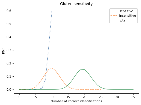
The results are the distributions for the number of correct identifications in each group.
Now we can use
add_dist to compute the distribution of the total number of correct identifications:
dist_total = Pmf.add_dist(dist_sensitive, dist_insensitive)
dist_sensitive.plot(label='sensitive', ls=':')
dist_insensitive.plot(label='insensitive', ls='--')
dist_total.plot(label='total')

decorate(xlabel='Number of correct identifications',
         ylabel='PMF',
         title='Gluten sensitivity')
We expect most of the sensitive subjects to identify the gluten flour correctly. Of the 25 insensitive subjects, we expect about 10 to identify the gluten flour by chance. So we expect about 20 correct identifications in total.
This is the answer to the forward problem: given the number of sensitive subjects, we can compute the distribution of the data.
Section 6.7 The Inverse Problem
Now let’s solve the inverse problem: given the data, we’ll compute the posterior distribution of the number of sensitive subjects.
Here’s how. I’ll loop through the possible values of
num_sensitive and compute the distribution of the data for each:
import pandas as pd

table = pd.DataFrame()
for num_sensitive in range(0, n+1):
    num_insensitive = n - num_sensitive
    dist_sensitive = make_binomial(num_sensitive, 0.95)
    dist_insensitive = make_binomial(num_insensitive, 0.4)
    dist_total = Pmf.add_dist(dist_sensitive, dist_insensitive)
    table[num_sensitive] = dist_total
The loop enumerates the possible values of
num_sensitive. For each value, it computes the distribution of the total number of correct identifications, and stores the result as a column in a Pandas
DataFrame.
0             1             2             3             4   \
0  1.719071e-08  1.432559e-09  1.193799e-10  9.948326e-12  8.290272e-13
1  4.011165e-07  5.968996e-08  7.162795e-09  7.792856e-10  8.013930e-11
2  4.545987e-06  9.741401e-07  1.709122e-07  2.506426e-08  3.269131e-09

             5             6             7             8             9   ...  \
0  6.908560e-14  5.757133e-15  4.797611e-16  3.998009e-17  3.331674e-18  ...
1  7.944844e-12  7.676178e-13  7.276377e-14  6.796616e-15  6.274653e-16  ...
2  3.940182e-10  4.490244e-11  4.908756e-12  5.197412e-13  5.365476e-14  ...

             26            27            28            29            30  \
0  1.501694e-36  1.251411e-37  1.042843e-38  8.690357e-40  7.241964e-41
1  7.508469e-34  6.486483e-35  5.596590e-36  4.823148e-37  4.152060e-38
2  1.806613e-31  1.620070e-32  1.449030e-33  1.292922e-34  1.151034e-35

             31            32            33            34            35
0  6.034970e-42  5.029142e-43  4.190952e-44  3.492460e-45  2.910383e-46
1  3.570691e-39  3.067777e-40  2.633315e-41  2.258457e-42  1.935405e-43
2  1.022555e-36  9.066202e-38  8.023344e-39  7.088005e-40  6.251357e-41

[3 rows x 36 columns]
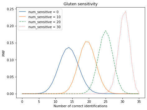
The following figure shows selected columns from the
DataFrame, corresponding to different hypothetical values of
num_sensitive:
table[0].plot(label='num_sensitive = 0')
table[10].plot(label='num_sensitive = 10')
table[20].plot(label='num_sensitive = 20', ls='--')
table[30].plot(label='num_sensitive = 30', ls=':')

decorate(xlabel='Number of correct identifications',
         ylabel='PMF',
         title='Gluten sensitivity')
Now we can use this table to compute the likelihood of the data:
likelihood1 = table.loc[12]
loc selects a row from the
DataFrame. The row with index 12 contains the probability of 12 correct identifications for each hypothetical value of
num_sensitive. And that’s exactly the likelihood we need to do a Bayesian update.
I’ll use a uniform prior, which implies that I would be equally surprised by any value of
num_sensitive:
hypos = np.arange(n+1)
prior = Pmf(1, hypos)
posterior1 = prior * likelihood1
posterior1.normalize()
0.4754741648615131
For comparison, I also compute the posterior for another possible outcome, 20 correct identifications.
likelihood2 = table.loc[20]
posterior2 = prior * likelihood2
posterior2.normalize()
1.7818649765887378
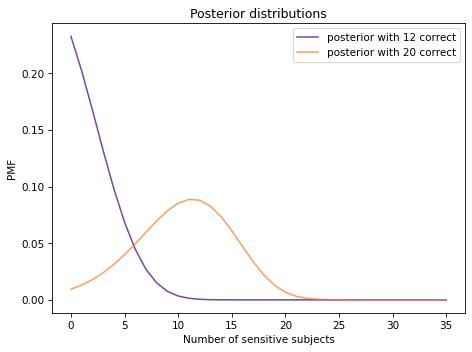
The following figure shows posterior distributions of
num_sensitive based on the actual data, 12 correct identifications, and the other possible outcome, 20 correct identifications.
posterior1.plot(label='posterior with 12 correct', color='C4')
posterior2.plot(label='posterior with 20 correct', color='C1')

decorate(xlabel='Number of sensitive subjects',
         ylabel='PMF',
         title='Posterior distributions')
With 12 correct identifications, the most likely conclusion is that none of the subjects are sensitive to gluten. If there had been 20 correct identifications, the most likely conclusion would be that 11-12 of the subjects were sensitive.
0
11