In the previous chapter we solved problems that involve estimating proportions. In the Euro problem, we estimated the probability that a coin lands heads up, and in the exercises, you estimated a batting average, the fraction of people who cheat on their taxes, and the chance of shooting down an invading alien.
Clearly, some of these problems are more realistic than others, and some are more useful than others.
In this chapter, we’ll work on problems related to counting, or estimating the size of a population. Again, some of the examples will seem silly, but some of them, like the German Tank problem, have real applications, sometimes in life and death situations.
Section 5.1 The Train Problem
"A railroad numbers its locomotives in order 1..N. One day you see a locomotive with the number 60. Estimate how many locomotives the railroad has."
Based on this observation, we know the railroad has 60 or more locomotives. But how many more? To apply Bayesian reasoning, we can break this problem into two steps:
-
What did we know about
\(N\) before we saw the data?
-
For any given value of
\(N\text{,}\) what is the likelihood of seeing the data (a locomotive with number 60)?
The answer to the first question is the prior. The answer to the second is the likelihood.
We don’t have much basis to choose a prior, so we’ll start with something simple and then consider alternatives. Let’s assume that
\(N\) is equally likely to be any value from 1 to 1000.
Here’s the prior distribution:
import numpy as np
from empiricaldist import Pmf

hypos = np.arange(1, 1001)
prior = Pmf(1, hypos)
Now let’s figure out the likelihood of the data. In a hypothetical fleet of
\(N\) locomotives, what is the probability that we would see number 60? If we assume that we are equally likely to see any locomotive, the chance of seeing any particular one is
\(1/N\text{.}\)
Here’s the function that does the update:
def update_train(pmf, data):
    """Update pmf based on new data."""
    hypos = pmf.qs
    likelihood = 1 / hypos
    impossible = (data > hypos)
    likelihood[impossible] = 0
    pmf *= likelihood
    pmf.normalize()
This function might look familiar; it is the same as the update function for the dice problem in the previous chapter. In terms of likelihood, the train problem is the same as the dice problem.
data = 60
posterior = prior.copy()
update_train(posterior, data)
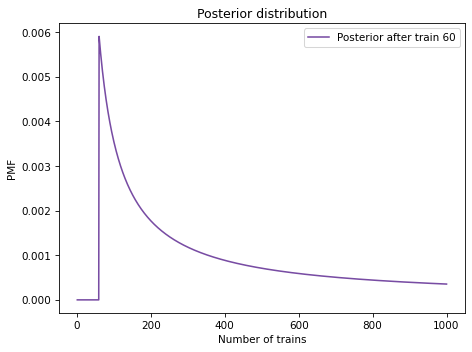
Here’s what the posterior looks like:
from utils import decorate

posterior.plot(label='Posterior after train 60', color='C4')
decorate(xlabel='Number of trains',
         ylabel='PMF',
         title='Posterior distribution')
Not surprisingly, all values of
\(N\) below 60 have been eliminated.
The most likely value, if you had to guess, is 60.
60
That might not seem like a very good guess; after all, what are the chances that you just happened to see the train with the highest number? Nevertheless, if you want to maximize the chance of getting the answer exactly right, you should guess 60.
But maybe that’s not the right goal. An alternative is to compute the mean of the posterior distribution. Given a set of possible quantities,
\(q_i\text{,}\) and their probabilities,
\(p_i\text{,}\) the mean of the distribution is:
\begin{equation*}
\mathrm{mean} = \sum_i p_i q_i
\end{equation*}
Which we can compute like this:
np.sum(posterior.ps * posterior.qs)
333.41989326370776
Or we can use the method provided by
Pmf:
333.41989326370776
The mean of the posterior is 333, so that might be a good guess if you want to minimize error. If you played this guessing game over and over, using the mean of the posterior as your estimate would minimize the
mean squared error over the long run.
Section 5.2 Sensitivity to the Prior
The prior I used in the previous section is uniform from 1 to 1000, but I offered no justification for choosing a uniform distribution or that particular upper bound. We might wonder whether the posterior distribution is sensitive to the prior. With so little data—only one observation—it is.
This table shows what happens as we vary the upper bound:
import pandas as pd

df = pd.DataFrame(columns=['Posterior mean'])
df.index.name = 'Upper bound'

for high in [500, 1000, 2000]:
    hypos = np.arange(1, high+1)
    pmf = Pmf(1, hypos)
    update_train(pmf, data=60)
    df.loc[high] = pmf.mean()

df
Posterior mean
Upper bound
500              207.079228
1000             333.419893
2000             552.179017
As we vary the upper bound, the posterior mean changes substantially. So that’s bad.
When the posterior is sensitive to the prior, there are two ways to proceed:
-
-
Get more background information and choose a better prior.
With more data, posterior distributions based on different priors tend to converge. For example, suppose that in addition to train 60 we also see trains 30 and 90.
Here’s how the posterior means depend on the upper bound of the prior, when we observe three trains:
df = pd.DataFrame(columns=['Posterior mean'])
df.index.name = 'Upper bound'

dataset = [30, 60, 90]

for high in [500, 1000, 2000]:
    hypos = np.arange(1, high+1)
    pmf = Pmf(1, hypos)
    for data in dataset:
        update_train(pmf, data)
    df.loc[high] = pmf.mean()

df
Posterior mean
Upper bound
500              151.849588
1000             164.305586
2000             171.338181
The differences are smaller, but apparently three trains are not enough for the posteriors to converge.
Section 5.3 Power Law Prior
If more data are not available, another option is to improve the priors by gathering more background information. It is probably not reasonable to assume that a train-operating company with 1000 locomotives is just as likely as a company with only 1.
With some effort, we could probably find a list of companies that operate locomotives in the area of observation. Or we could interview an expert in rail shipping to gather information about the typical size of companies.
But even without getting into the specifics of railroad economics, we can make some educated guesses. In most fields, there are many small companies, fewer medium-sized companies, and only one or two very large companies.
This law suggests that if there are 1000 companies with fewer than 10 locomotives, there might be 100 companies with 100 locomotives, 10 companies with 1000, and possibly one company with 10,000 locomotives.
Mathematically, a power law means that the number of companies with a given size,
\(N\text{,}\) is proportional to
\((1/N)^{\alpha}\text{,}\) where
\(\alpha\) is a parameter that is often near 1.
We can construct a power law prior like this:
alpha = 1.0
ps = hypos**(-alpha)
power = Pmf(ps, hypos, name='power law')
power.normalize()
8.178368103610282
For comparison, here’s the uniform prior again.
hypos = np.arange(1, 1001)
uniform = Pmf(1, hypos, name='uniform')
uniform.normalize()
1000
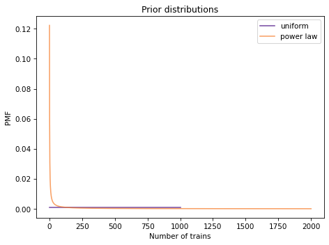
Here’s what a power law prior looks like, compared to the uniform prior:
uniform.plot(color='C4')
power.plot(color='C1')

decorate(xlabel='Number of trains',
         ylabel='PMF',
         title='Prior distributions')
Here’s the update for both priors.
dataset = [60]
for data in dataset:
    update_train(uniform, data)
    update_train(power, data)
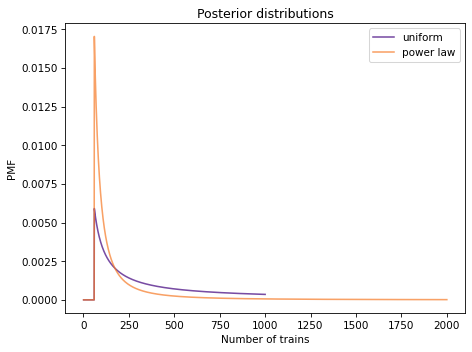
And here are the posterior distributions.
uniform.plot(color='C4')
power.plot(color='C1')

decorate(xlabel='Number of trains',
         ylabel='PMF',
         title='Posterior distributions')
The power law gives less prior probability to high values, which yields lower posterior means, and less sensitivity to the upper bound.
Here’s how the posterior means depend on the upper bound when we use a power law prior and observe three trains:
df = pd.DataFrame(columns=['Posterior mean'])
df.index.name = 'Upper bound'

alpha = 1.0
dataset = [30, 60, 90]

for high in [500, 1000, 2000]:
    hypos = np.arange(1, high+1)
    ps = hypos**(-alpha)
    power = Pmf(ps, hypos)
    for data in dataset:
        update_train(power, data)
    df.loc[high] = power.mean()

df
Posterior mean
Upper bound
500              130.708470
1000             133.275231
2000             133.997463
Now the differences are much smaller. In fact, with an arbitrarily large upper bound, the mean converges on 134.
So the power law prior is more realistic, because it is based on general information about the size of companies, and it behaves better in practice.
Section 5.4 Credible Intervals
So far we have seen two ways to summarize a posterior distribution: the value with the highest posterior probability (the MAP) and the posterior mean. These are both
point estimates, that is, single values that estimate the quantity we are interested in.
Another way to summarize a posterior distribution is with percentiles. If you have taken a standardized test, you might be familiar with percentiles. For example, if your score is the 90th percentile, that means you did as well as or better than 90% of the people who took the test.
If we are given a value,
x, we can compute its
percentile rank by finding all values less than or equal to
x and adding up their probabilities.
Pmf provides a method that does this computation. So, for example, we can compute the probability that the company has less than or equal to 100 trains:
0.2937469222495771
With a power law prior and a dataset of three trains, the result is about 29%. So 100 trains is the 29th percentile.
Going the other way, suppose we want to compute a particular percentile; for example, the median of a distribution is the 50th percentile. We can compute it by adding up probabilities until the total exceeds 0.5. Here’s a function that does it:
def quantile(pmf, prob):
    """Compute a quantile with the given prob."""
    total = 0
    for q, p in pmf.items():
        total += p
        if total >= prob:
            return q
    return np.nan
The loop uses
items, which iterates the quantities and probabilities in the distribution. Inside the loop we add up the probabilities of the quantities in order. When the total equals or exceeds
prob, we return the corresponding quantity.
This function is called
quantile because it computes a quantile rather than a percentile. The difference is the way we specify
prob. If
prob is a percentage between 0 and 100, we call the corresponding quantity a percentile. If
prob is a probability between 0 and 1, we call the corresponding quantity a
quantile.
Here’s how we can use this function to compute the 50th percentile of the posterior distribution:
113
The result, 113 trains, is the median of the posterior distribution.
Pmf provides a method called
quantile that does the same thing. We can call it like this to compute the 5th and 95th percentiles:
power.quantile([0.05, 0.95])
array([ 91., 243.])
The result is the interval from 91 to 243 trains, which implies:
-
The probability is 5% that the number of trains is less than or equal to 91.
-
The probability is 5% that the number of trains is greater than 243.
Therefore the probability is 90% that the number of trains falls between 91 and 243 (excluding 91 and including 243). For this reason, this interval is called a 90%
credible interval.
Pmf also provides
credible_interval, which computes an interval that contains the given probability.
power.credible_interval(0.9)
array([ 91., 243.])
Section 5.5 The German Tank Problem
During World War II, the Economic Warfare Division of the American Embassy in London used statistical analysis to estimate German production of tanks and other equipment.
The Western Allies had captured log books, inventories, and repair records that included chassis and engine serial numbers for individual tanks.
Analysis of these records indicated that serial numbers were allocated by manufacturer and tank type in blocks of 100 numbers, that numbers in each block were used sequentially, and that not all numbers in each block were used. So the problem of estimating German tank production could be reduced, within each block of 100 numbers, to a form of the train problem.
Based on this insight, American and British analysts produced estimates substantially lower than estimates from other forms of intelligence. And after the war, records indicated that they were substantially more accurate.
They performed similar analyses for tires, trucks, rockets, and other equipment, yielding accurate and actionable economic intelligence.
The German tank problem is historically interesting; it is also a nice example of real-world application of statistical estimation.
For more on this problem, see
this Wikipedia page and Ruggles and Brodie, "An Empirical Approach to Economic Intelligence in World War II",
Journal of the American Statistical Association, March 1947,
available here.