Section 18.1 The World Cup Problem Revisited
In
Chapter 8, we solved the World Cup problem using a Poisson process to model goals in a soccer game as random events that are equally likely to occur at any point during a game.
We used a gamma distribution to represent the prior distribution of
\(\lambda\text{,}\) the goal-scoring rate. And we used a Poisson distribution to compute the probability of
\(k\text{,}\) the number of goals scored.
Here’s a gamma object that represents the prior distribution.
from scipy.stats import gamma

alpha = 1.4
dist = gamma(alpha)
And here’s a grid approximation.
import numpy as np
from utils import pmf_from_dist

lams = np.linspace(0, 10, 101)
prior = pmf_from_dist(dist, lams)
Here’s the likelihood of scoring 4 goals for each possible value of
lam.
from scipy.stats import poisson

k = 4
likelihood = poisson(lams).pmf(k)
posterior = prior * likelihood
posterior.normalize()
0.05015532557804499
So far, this should be familiar. Now we’ll solve the same problem using the conjugate prior.
Section 18.2 The Conjugate Prior
In
Section 8.3, I presented three reasons to use a gamma distribution for the prior and said there was a fourth reason I would reveal later. Well, now is the time.
The other reason I chose the gamma distribution is that it is the "conjugate prior" of the Poisson distribution, so-called because the two distributions are connected or coupled, which is what "conjugate" means.
In the next section I’ll explain
how they are connected, but first I’ll show you the consequence of this connection, which is that there is a remarkably simple way to compute the posterior distribution.
However, in order to demonstrate it, we have to switch from the one-parameter version of the gamma distribution to the two-parameter version. Since the first parameter is called
alpha, you might guess that the second parameter is called
beta.
The following function takes
alpha and
beta and makes an object that represents a gamma distribution with those parameters.
def make_gamma_dist(alpha, beta):
    """Makes a gamma object."""
    dist = gamma(alpha, scale=1/beta)
    dist.alpha = alpha
    dist.beta = beta
    return dist
Here’s the prior distribution with
alpha=1.4 again and
beta=1.
alpha = 1.4
beta = 1

prior_gamma = make_gamma_dist(alpha, beta)
prior_gamma.mean()
1.4
Now I claim without proof that we can do a Bayesian update with
k goals just by making a gamma distribution with parameters
alpha+k and
beta+1.
def update_gamma(prior, data):
    """Update a gamma prior."""
    k, t = data
    alpha = prior.alpha + k
    beta = prior.beta + t
    return make_gamma_dist(alpha, beta)
Here’s how we update it with
k=4 goals in
t=1 game.
data = 4, 1
posterior_gamma = update_gamma(prior_gamma, data)
After all the work we did with the grid, it might seem absurd that we can do a Bayesian update by adding two pairs of numbers. So let’s confirm that it works.
I’ll make a
Pmf with a discrete approximation of the posterior distribution.
posterior_conjugate = pmf_from_dist(posterior_gamma, lams)
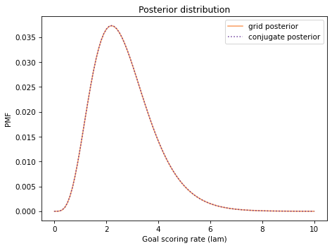
The following figure shows the result along with the posterior we computed using the grid algorithm.
from utils import decorate

def decorate_rate(title=''):
    decorate(xlabel='Goal scoring rate (lam)',
             ylabel='PMF',
             title=title)
posterior.plot(label='grid posterior', color='C1')
posterior_conjugate.plot(label='conjugate posterior',
                         color='C4', ls=':')

decorate_rate('Posterior distribution')
They are the same other than small differences due to floating-point approximations.
np.allclose(posterior, posterior_conjugate)
True
Section 18.3 What the Actual?
To understand how that works, we’ll write the PDF of the gamma prior and the PMF of the Poisson likelihood, then multiply them together, because that’s what the Bayesian update does. We’ll see that the result is a gamma distribution, and we’ll derive its parameters.
Here’s the PDF of the gamma prior, which is the probability density for each value of
\(\lambda\text{,}\) given parameters
\(\alpha\) and
\(\beta\text{:}\)
\begin{equation*}
\lambda^{\alpha-1} e^{-\lambda \beta}
\end{equation*}
I have omitted the normalizing factor; since we are planning to normalize the posterior distribution anyway, we don’t really need it.
Now suppose a team scores
\(k\) goals in
\(t\) games. The probability of this data is given by the PMF of the Poisson distribution, which is a function of
\(k\) with
\(\lambda\) and
\(t\) as parameters.
\begin{equation*}
\lambda^k e^{-\lambda t}
\end{equation*}
Again, I have omitted the normalizing factor, which makes it clearer that the gamma and Poisson distributions have the same functional form. When we multiply them together, we can pair up the factors and add up the exponents. The result is the unnormalized posterior distribution,
\begin{equation*}
\lambda^{\alpha-1+k} e^{-\lambda(\beta + t)}
\end{equation*}
which we can recognize as an unnormalized gamma distribution with parameters
\(\alpha + k\) and
\(\beta + t\text{.}\)
This derivation provides insight into what the parameters of the posterior distribution mean:
\(\alpha\) reflects the number of events that have occurred;
\(\beta\) reflects the elapsed time.
Section 18.4 Binomial Likelihood
As a second example, let’s look again at the Euro problem. When we solved it with a grid algorithm, we started with a uniform prior:
from utils import make_uniform

xs = np.linspace(0, 1, 101)
uniform = make_uniform(xs, 'uniform')
We used the binomial distribution to compute the likelihood of the data, which was 140 heads out of 250 attempts.
from scipy.stats import binom

k, n = 140, 250
xs = uniform.qs
likelihood = binom.pmf(k, n, xs)
Then we computed the posterior distribution in the usual way.
posterior = uniform * likelihood
posterior.normalize()
0.003944617569326651
We can solve this problem more efficiently using the conjugate prior of the binomial distribution, which is the beta distribution.
The beta distribution is bounded between 0 and 1, so it works well for representing the distribution of a probability like
x. It has two parameters, called
alpha and
beta, that determine the shape of the distribution.
SciPy provides an object called
beta that represents a beta distribution. The following function takes
alpha and
beta and returns a new
beta object.
import scipy.stats

def make_beta(alpha, beta):
    """Makes a beta object."""
    dist = scipy.stats.beta(alpha, beta)
    dist.alpha = alpha
    dist.beta = beta
    return dist
It turns out that the uniform distribution, which we used as a prior, is the beta distribution with parameters
alpha=1 and
beta=1. So we can make a
beta object that represents a uniform distribution, like this:
alpha = 1
beta = 1

prior_beta = make_beta(alpha, beta)
Now let’s figure out how to do the update. As in the previous example, we’ll write the PDF of the prior distribution and the PMF of the likelihood function, and multiply them together. We’ll see that the product has the same form as the prior, and we’ll derive its parameters.
Here is the PDF of the beta distribution, which is a function of
\(x\) with
\(\alpha\) and
\(\beta\) as parameters.
\begin{equation*}
x^{\alpha-1} (1-x)^{\beta-1}
\end{equation*}
Again, I have omitted the normalizing factor, which we don’t need because we are going to normalize the distribution after the update.
And here’s the PMF of the binomial distribution, which is a function of
\(k\) with
\(n\) and
\(x\) as parameters.
\begin{equation*}
x^{k} (1-x)^{n-k}
\end{equation*}
Again, I have omitted the normalizing factor. Now when we multiply the beta prior and the binomial likelihood, the result is
\begin{equation*}
x^{\alpha-1+k} (1-x)^{\beta-1+n-k}
\end{equation*}
which we recognize as an unnormalized beta distribution with parameters
\(\alpha+k\) and
\(\beta+n-k\text{.}\)
So if we observe
k successes in
n trials, we can do the update by making a beta distribution with parameters
alpha+k and
beta+n-k. That’s what this function does:
def update_beta(prior, data):
    """Update a beta distribution."""
    k, n = data
    alpha = prior.alpha + k
    beta = prior.beta + n - k
    return make_beta(alpha, beta)
Again, the conjugate prior gives us insight into the meaning of the parameters;
\(\alpha\) is related to the number of observed successes;
\(\beta\) is related to the number of failures.
Here’s how we do the update with the observed data.
data = 140, 250
posterior_beta = update_beta(prior_beta, data)
To confirm that it works, I’ll evaluate the posterior distribution for the possible values of
xs and put the results in a
Pmf.
posterior_conjugate = pmf_from_dist(posterior_beta, xs)
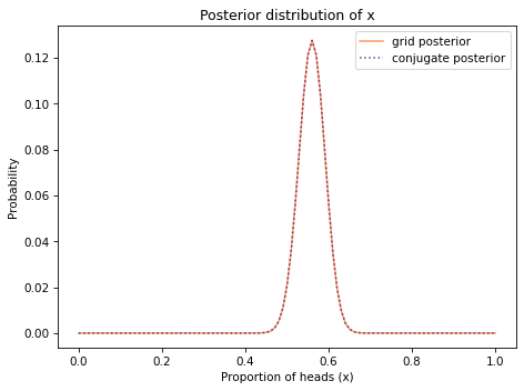
And we can compare the posterior distribution we just computed with the results from the grid algorithm.
def decorate_euro(title):
    decorate(xlabel='Proportion of heads (x)',
             ylabel='Probability',
             title=title)
posterior.plot(label='grid posterior', color='C1')
posterior_conjugate.plot(label='conjugate posterior',
                        color='C4', ls=':')

decorate_euro(title='Posterior distribution of x')
They are the same other than small differences due to floating-point approximations.
The examples so far are problems we have already solved, so let’s try something new.
np.allclose(posterior, posterior_conjugate)
True
Section 18.5 Lions and Tigers and Bears
Suppose we visit a wild animal preserve where we know that the only animals are lions and tigers and bears, but we don’t know how many of each there are. During the tour, we see 3 lions, 2 tigers, and one bear. Assuming that every animal had an equal chance to appear in our sample, what is the probability that the next animal we see is a bear?
To answer this question, we’ll use the data to estimate the prevalence of each species, that is, what fraction of the animals belong to each species. If we know the prevalences, we can use the multinomial distribution to compute the probability of the data. For example, suppose we know that the fraction of lions, tigers, and bears is 0.4, 0.3, and 0.3, respectively.
In that case the probability of the data is:
from scipy.stats import multinomial

data = 3, 2, 1
n = np.sum(data)
ps = 0.4, 0.3, 0.3

multinomial.pmf(data, n, ps)
0.10368
Now, we could choose a prior for the prevalences and do a Bayesian update using the multinomial distribution to compute the probability of the data.
But there’s an easier way, because the multinomial distribution has a conjugate prior: the Dirichlet distribution.
Section 18.6 The Dirichlet Distribution
The Dirichlet distribution is a multivariate distribution, like the multivariate normal distribution we used in
Section 12.6 to describe the distribution of penguin measurements.
In that example, the quantities in the distribution are pairs of flipper length and culmen length, and the parameters of the distribution are a vector of means and a matrix of covariances.
In a Dirichlet distribution, the quantities are vectors of probabilities,
\(\mathbf{x}\text{,}\) and the parameter is a vector,
\(\mathbf{\alpha}\text{.}\)
An example will make that clearer. SciPy provides a
dirichlet object that represents a Dirichlet distribution. Here’s an instance with
\(\mathbf{\alpha} = 1, 2, 3\text{.}\)
from scipy.stats import dirichlet

alpha = 1, 2, 3
dist = dirichlet(alpha)
Since we provided three parameters, the result is a distribution of three variables. If we draw a random value from this distribution, like this:
array([[0.00389931, 0.49015107, 0.50594962]])
1.0000000000000002
The result is an array of three values. They are bounded between 0 and 1, and they always add up to 1, so they can be interpreted as the probabilities of a set of outcomes that are mutually exclusive and collectively exhaustive.
Let’s see what the distributions of these values look like. I’ll draw 1000 random vectors from this distribution, like this:
(1000, 3)
The result is an array with 1000 rows and three columns. I’ll compute the
Cdf of the values in each column.
from empiricaldist import Cdf

cdfs = [Cdf.from_seq(col)
        for col in sample.transpose()]
The result is a list of
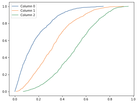
Cdf objects that represent the marginal distributions of the three variables. Here’s what they look like.
for i, cdf in enumerate(cdfs):
    label = f'Column {i}'
    cdf.plot(label=label)

decorate()
Column 0, which corresponds to the lowest parameter, contains the lowest probabilities. Column 2, which corresponds to the highest parameter, contains the highest probabilities.
As it turns out, these marginal distributions are beta distributions. The following function takes a sequence of parameters,
alpha, and computes the marginal distribution of variable
i:
def marginal_beta(alpha, i):
    """Compute the ith marginal of a Dirichlet distribution."""
    total = np.sum(alpha)
    return make_beta(alpha[i], total-alpha[i])
We can use it to compute the marginal distribution for the three variables.
marginals = [marginal_beta(alpha, i)
             for i in range(len(alpha))]
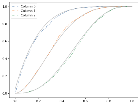
The following plot shows the CDF of these distributions as gray lines and compares them to the CDFs of the samples.
xs = np.linspace(0, 1, 101)

for i in range(len(alpha)):
    label = f'Column {i}'

    pmf = pmf_from_dist(marginals[i], xs)
    pmf.make_cdf().plot(color='C5')

    cdf = cdfs[i]
    cdf.plot(label=label, ls=':')

decorate()
This confirms that the marginals of the Dirichlet distribution are beta distributions. And that’s useful because the Dirichlet distribution is the conjugate prior for the multinomial likelihood function.
If the prior distribution is Dirichlet with parameter vector
alpha and the data is a vector of observations,
data, the posterior distribution is Dirichlet with parameter vector
alpha + data.
As an exercise at the end of this chapter, you can use this method to solve the Lions and Tigers and Bears problem.