Section 8.3 Analysis of Variance (ANOVA)
Subsection 8.3.1 Introduction
1
This subsection is adapted from David M. Lane. “Introduction.” Online Statistics Education: A Multimedia Course of Study. https://onlinestatbook.com/2/analysis_of_variance/intro.html
Analysis of Variance (ANOVA)is a statistical method used to test differences between two or more means. It may seem odd that the technique is called “Analysis of Variance” rather than “Analysis of Means.” The name is appropriate because inferences about means are made by analyzing variance, as outlined in this chapter’s appendix.
ANOVA is used to test general rather than specific differences among means. This can be seen best by example, so we will continue considering the data on leniency and smiles we examined in the prior section on the Tukey HSD test.
ANOVA tests the non-specific null hypothesis that all four population means are equal. That is,
\begin{equation*}
\mu_{false} = \mu_{felt} = \mu_{miserable} = \mu_{neutral}
\end{equation*}
in our example. More generally, the null hypothesis tested by ANOVA is that the population means for all conditions are the same. For whatever data is being examined, this can be written as:
\begin{equation*}
H_0: \mu_1 = \mu_2 = ... = \mu_k
\end{equation*}
where \(H_0\) is the null hypothesis and k is the number of conditions (k = 4 in our example).
This non-specific null hypothesis is sometimes called the omnibus null hypothesis. When the omnibus null hypothesis is rejected, the conclusion is that at least one population mean is different from at least one other mean. However, since the ANOVA does not reveal which means are different from which, it offers less specific information than the Tukey HSD test. The Tukey HSD is therefore preferable to ANOVA in this situation.
You might be wondering why you should learn about ANOVA when the Tukey test is better. One reason is that there are complex types of analyses that can be done with ANOVA and not with the Tukey test. A second is that ANOVA is one of the most commonly-used technique for comparing means, and it is important to understand ANOVA in order to understand research reports.
Subsection 8.3.2 The Critical Step: Calculating an F Ratio
2
This subsection and the following are adapted from David M. Lane. “One-Factor ANOVA (Between Subjects).” Online Statistics Education: A Multimedia Course of Study. https://onlinestatbook.com/2/analysis_of_variance/one-way.html
There are many types of ANOVA, but for our example, we will use what is called a one-factor between-subjects design. Other types of ANOVA are beyond the scope of what is covered in this text.
More details are provided in this chapter’s appendix, but the critical step in an ANOVA is comparing what is called the mean square error (MSE) to the mean square between (MSB). MSB estimates a larger quantity than MSE only when the population means are not equal, so finding a larger MSB than an MSE is a sign that the population means are not equal. But since MSB could be larger than MSE by chance even if the population means are equal, MSB must be much larger than MSE in order to justify the conclusion that the population means differ. But how much larger must MSB be? For the “Smiles and Leniency” data, the MSB and MSE are 9.179 and 2.649, respectively. Is that difference big enough? To answer, we would need to know the probability of getting that big a difference or a bigger difference if the population means were all equal. The mathematics necessary to answer this question were worked out by the statistician R. Fisher. Although Fisher’s original formulation took a slightly different form, the standard method for determining the probability is based on the ratio of MSB to MSE. This ratio is named after Fisher and is called the F ratio.
For these data, the F ratio is
\begin{equation*}
F = \frac{9.179}{2.649} = 3.465.
\end{equation*}
Therefore, the MSB is 3.465 times higher than MSE. Would this have been likely to happen if all the population means were equal? That depends on the sample size. With a small sample size, it would not be too surprising because results from small samples are unstable. However, with a very large sample, the MSB and MSE are almost always about the same (assuming the null hypothesis is true), and an F ratio of 3.465 or larger would be very unusual.Figure 8.5shows the sampling distribution of F for the sample size in the “Smiles and Leniency” study. As you can see, it has a positive skew.
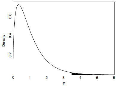
FromFigure 8.5, you can see that F ratios of 3.465 or above are unusual occurrences. The area to the right of 3.465 represents the probability of an F that large or larger and is equal to 0.018. In other words, given the null hypothesis that all the population means are equal, the probability value (p) is 0.018 and therefore the null hypothesis can be rejected. The conclusion that at least one of the population means is different from at least one of the others is justified.
The shape of the F distribution depends on the sample size. More precisely, it depends on two degrees of freedom (df) parameters: one for the numerator (MSB) and one for the denominator (MSE). Recall that the degrees of freedom for an estimate of variance is equal to the number of observations minus one. Since the MSB is the variance of k means (where k is the number of groups), it has k - 1 df. The MSE is an average of k variances, each with n - 1 df. Therefore, the df for MSE is k(n - 1) = N - k, where N is the total number of observations, n is the number of observations in each group, and k is the number of groups. To summarize:
\begin{equation*}
df_{\text{numerator}} = k-1
\end{equation*}
\begin{equation*}
df_{\text{denominator}} = N-k
\end{equation*}
For the “Smiles and Leniency” data,
\begin{equation*}
df_{\text{numerator}} = k-1 = 4-1 = 3
\end{equation*}
\begin{equation*}
df_{\text{denominator}} = N-k = 136-4 = 132
\end{equation*}
\begin{equation*}
F = 3.465
\end{equation*}
An F distribution calculator shows that p = 0.018. Again, because this value is less than 0.05, one would generally reject the null hypothesis and conclude that average leniency varies depending on type of smile. The p-value from an ANOVA is sometimes reported in a larger table of summary results such as Table 8.7.
| Source | df | SSQ | MS | F | p |
|---|---|---|---|---|---|
| Condition | 3 | 27.5349 | 9.1783 | 3.465 | 0.0182 |
| Error | 132 | 349.6544 | 2.6489 | ||
| Total | 135 | 377.1893 |
Subsection 8.3.3 Relationship to T Tests and Regression
Since an ANOVA and an independent-groups t test can both test the difference between two means, you might be wondering which one to use. Fortunately, it does not matter since the results will always be the same. When there are only two groups, the following relationship between F and t will always hold:
\begin{equation*}
F(1,dfd) = t^2(df)
\end{equation*}
where dfd is the degrees of freedom for the denominator of the F test and df is the degrees of freedom for the t test. dfd will always equal df. And because of how their probability distributions are constructed, these values of F and t will yield identical p-values for the (two tailed) null hypothesis of no difference between the two means.
There is also a third equivalent way to compare two means: using regression, as described in Chapter 12. More generally, regression and ANOVA are two sides of the same coin and will yield equivalent results (assuming the same data/assumptions), even when testing for differences among more than two means. Statistical software will generally include a model F statistic among the results shown for a regression, and in the case of a model a single qualitative independent variable, the regression model F statistic will be the same F ratio used in an ANOVA. Because of this equivalence, whether one reports results as an ANOVA or regression is usually a matter of habit and familiarity. In some social science literatures, ANOVA results are rarely reported because researchers typically default to using regression instead.

