Section 12.1 Predicting extroversion using gender
If I want to describe differences in extroversion by gender in this dataset, I can compute the mean value of extroversion for males and for females. It turns out that males have an average extroversion of -0.46 while females’ average level of extroversion is 0.53. Thus, the average female is about 1-point more extroverted than the average male. But of course, there is abundant variation in extroversion among both groups, as seen clearly in Figure 12.1.1. There are plenty of females who are introverts and plenty of males who are extroverts.
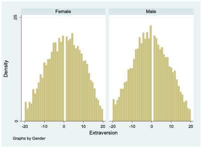
If you asked me to guess the extroversion level of someone in this dataset and the only thing you told me about them was their gender, my best bet would probably be to guess the average extroversion level for someone of that gender. So for a female I knew nothing else about, I would guess their extroversion to be 0.53, while for a male I’d guess -0.46.
When we’re working with data, sometimes it’s helpful to express how I would make a guess about a dependent variable (extroversion) based on an independent variable (gender) using a mathematical formula. In fact, this is exactly what we do when we run a regression. There are many ways I could write this formula, but I’ll show just two for now. First, I could write:
\begin{equation}
\widehat{Extraversion}=0.53 \times Female-0.46 \times Male\tag{12.1.1}
\end{equation}
Notice I’ve added a “hat” above the name of the variable Extraversion; this hat means that I’m making a guess about the value of that variable (I’m guessing the level of extroversion based on gender). The equation has two other variables Female and Male, and these two variables will take on a value of 1 if the person’s gender is equal to the name of the variable and will otherwise take on a value of 0. For a female, Female will equal 1 and Male will equal 0, giving us:
\begin{equation*}
\widehat{Extraversion}=0.53 \times (1)-0.46 \times (0)=0.53
\end{equation*}
So our guess for the level of extroversion (\(\widehat{Extraversion}\)) of a female we know nothing about is 0.53.
For a male, our guess is:
\begin{equation*}
\widehat{Extraversion}=0.53 \times (0)-0.46 \times (1)=-0.46
\end{equation*}
There’s a second way I can write my formula, which will turn out to be more useful in the future when we come to consider multiple factors at the same time that might help us predict the value of a dependent variable. Rather than having two variables to represent gender in my equation, I can just use one:
\begin{equation}
\widehat{Extraversion}=0.53-0.99 \times Male\tag{12.1.2}
\end{equation}
In (12.1.2), we start from female as our baseline. Notice that the first number we see (0.53) is our guess for the value of extroversion for a female. When we’re considering a female, Male=0, so:
\begin{equation*}
\widehat{Extraversion}=0.53-0.99 \times 0=0.53
\end{equation*}
Thus, we get the right prediction for females from this equation, even though we didn’t include a variable specifically for females. If we have a male, Male=1, so we get:
\begin{equation*}
\widehat{Extraversion}=0.53-0.99 \times 1=-0.46
\end{equation*}
This is the same prediction we got before. Remember, I decided to initially just analyze respondents who selected either male or female. Since we are only considering two categories (male or female), and each respondent is either a male or a female, saying Male = 1 lets me know that Female = 0. It’s actually repetitive in this context to both say that Male = 1 and Female = 0. Similarly, saying Male = 0 implies that Female = 1. So I can simplify my equation by just including one variable to indicate binary gender.
Notice that in (12.1.2), the number next to Male is equal to the difference between the average level of extroversion for females and the average level for males (0.53-(-0.46)=0.99). This is because (12.1.2) starts with females as the baseline, so to get our prediction for males, we have to adjust our baseline prediction by the average difference for males.

