Section 4.2 Confidence Intervals: A Key Tool for Estimation
1
The beginning of this section is adapted from David M. Lane. "Confidence Intervals Introduction." Online Statistics Education: A Multimedia Course of Study. https://onlinestatbook.com/2/estimation/confidence.html
Say you were interested in the mean weight of 10-year-old girls living in the United States. Since it would have been impractical to weigh all the 10-year-old girls in the United States, you took a sample of 16 and found that the mean weight was 90 pounds. This sample mean of 90 is a point estimate of the population mean. A point estimate by itself is of limited usefulness because it does not reveal the uncertainty associated with the estimate; you do not have a good sense of how far this sample mean may be from the population mean. For example, can you be confident that the population mean is within 5 pounds of 90? You simply do not know.
Confidence intervals provide more information than point estimates. Confidence intervals for means are intervals constructed using a procedure that will contain the population mean a specified proportion of the time, typically either 95% or 99% of the time. These intervals are referred to as 95% and 99% confidence intervals respectively. An example of a 95% confidence interval is shown below:
\begin{equation*}
72.85 \lt \mu \lt 107.15
\end{equation*}
Based on this interval, there is good reason to believe that the population mean lies between these two bounds of 72.85 and 107.15 since 95% of the time confidence intervals contain the true mean.
If repeated samples were taken and the 95% confidence interval computed for each sample, 95% of the intervals would contain the population mean. Naturally, 5% of the intervals would not contain the population mean.
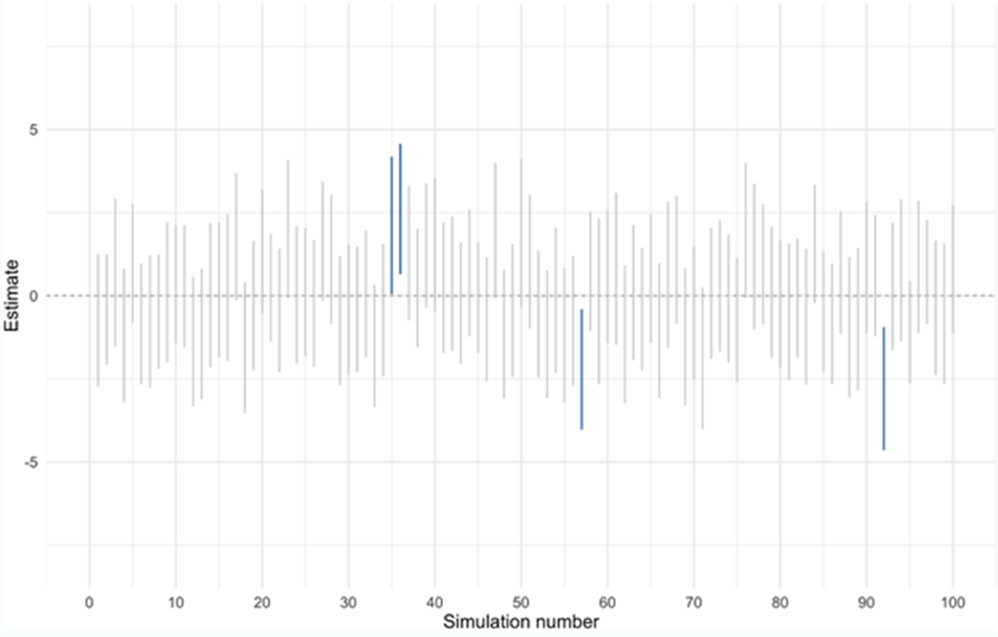
2
This image is shared under CC-BY 4.0 and is adapted from Figure 1 of Nalborczyk, L., Bürkner, P. C., & Williams, D. R. (2019). Pragmatism should not be a substitute for statistical literacy, a commentary on Albers, Kiers, and van Ravenzwaaij (2018). Journal of European Psychology Students, 10(1), 1-10.
This property of 95% confidence intervals is demonstrated in Figure 4.2.1, which shows the results of a simulation in which random samples were drawn again and again, to see how interval estimates behave. Suppose the population mean is zero and each vertical bar represents a different random sample and the resulting confidence interval. As you can see, most intervals overlap with the true population mean of zero (on the y axis), but we also expect one out of every 20 estimates (5%) to miss the mark (the bars shown in blue). In practice, we would normally only have one sample and wouldn’t know for sure if ours is one of the unlucky cases in which the confidence interval fails to include the population mean. What we do know is that we’ve followed a process that gives a correct answer 19 times out of 20.
What procedure is used to construct a confidence interval? We will learn the details in Chapter 6. For now, it is enough to know that there are well-established procedures for constructing confidence intervals in various settings. Even without knowing these exact procedures, you can hopefully begin to see the usefulness of confidence intervals from the examples in this chapter.
Note that confidence intervals can be computed for various parameters, not just the mean. In the following sections, we will see how confidence intervals can be applied to estimates of the difference in means as well as regression slope coefficients.
3
A parameter is a value calculated in a population. For example, the mean of the numbers in a population is a parameter. Compare with a sample statistic, which is a value computed in a sample to estimate a parameter. (https://onlinestatbook.com/2/glossary/parameter.html)
Subsection 4.2.1 A Practical Example: Estimating the Difference in Means
4
This subsection is adapted from David M. Lane. "Difference between Means." Online Statistics Education: A Multimedia Course of Study. https://onlinestatbook.com/2/estimation/difference_means.html
It is much more common for a researcher to be interested in the difference between means than in the specific values of the means themselves. Using statistical jargon introduced in the prior section, we could therefore say that the parameter of interest is often the difference in population means. We take as an example the data from the “Animal Research” case study. In this experiment, students rated (on a 7-point scale) whether they thought animal research is wrong. The sample sizes, means, and variances are shown separately for males and females in Table 4.2.2.
| Condition | n | Mean | Variance |
|---|---|---|---|
| Females | 17 | 5.353 | 2.743 |
| Males | 17 | 3.882 | 2.985 |
As you can see, the females rated animal research as more wrong than did the males. This sample difference between the female mean of 5.35 and the male mean of 3.88 is 1.47. However, the gender difference in this particular sample is not very important. What is important is the difference in the population. The difference in sample means is used to estimate the difference in population means. The accuracy of the estimate is revealed by a confidence interval.
In order to construct a confidence interval, we need to make some assumptions. The specifics might not make a lot of sense yet, but here are the three assumptions we need to make to obtain our confidence interval in this example:
-
The two populations have the same variance. This assumption is called the assumption of homogeneity of variance.
-
The populations are normally distributed.
-
Each value is sampled independently from each other value.
Using these assumptions, one can use a bunch of fancy math formulas (or statistical software) to get the following confidence interval:
\begin{equation*}
0.29 \leq \mu_f - \mu_m \leq 2.65
\end{equation*}
where \(\mu_f\) is the population mean for females and \(\mu_m\) is the population mean for males. Since the difference in these population means is the main parameter we wish to estimate, we could say the confidence interval for the parameter of interest is [0.29, 2.65]. Because all values within this range are positive, this analysis provides evidence that the mean for females is higher than the mean for males. More specifically, the difference between means in the population is likely to be between 0.29 and 2.65. Note that since 0 does not fall within the range of the confidence interval, this suggests that there is a difference between males and females, so we can also say that the results are statistically significant.
If, instead, we had found a confidence interval of [-1.03, 2.65], we could not rule out the possibility of no difference between males and females, since 0 falls between -1.03 and 2.65.
Subsection 4.2.2 Introducing Confidence Intervals for Regression
6
This subsection is written by Nathan Favero.
Let’s examine one more practical example of using confidence intervals, this time in the context of regression. For this example, we return to the regression results table presented at the end of the previous chapter (Section 3.5). The table is shown again here as Table 4.2.3.
| Coef. | Std. err. | p-value | |
|---|---|---|---|
| verb_sat | 0.0017 | 0.0010 | 0.10 |
| math_sat | 0.0048 | 0.0012 | 0.00014 |
| (intercept) | -0.91 | 0.42 | 0.033 |
| n | 105 | ||
| \(r^2\) | 0.487 |
Because the coefficients we see in the table are just point estimates, confidence intervals can help us better understand the precision of these estimates by providing us with a range of plausible values for the coefficients. Notice that no confidence intervals have been provided in the table (which is a situation you may frequently encounter when reading social scientific research publications). Fortunately, we can easily calculate a good approximation of a confidence interval for a coefficient estimate \(\hat{\beta_i}\) as long as we also have its standard error estimate (\(s_{\beta_i}\)), which is provided in the table (in the column label “Std. err.”). We will learn exactly what a standard error is in Chapter 6, but for now, we can simply insert the standard error estimate into the following formulas:
7
Some publications list t scores or z scores instead of standard errors. These t (or z) scores are typically just the coefficient divided by the standard error estimate, so you can obtain the standard error estimate by dividing the coefficient (\(\hat{\beta_i}\)) by its corresponding t score (or z score).
\begin{align*}
\text{Lower limit} \amp\approx \hat{\beta_i} - 2\times s_{\beta_i}\\
\text{Upper limit} \amp\approx \hat{\beta_i} + 2\times s_{\beta_i}
\end{align*}
Note that these formulas are just an approximation; the formulas for precise intervals are shown in a later chapter. In this approximation, all we are doing is multiplying the standard error by two to get the margin of error. From our initial point estimate of the slope, we can then add or subtract the margin of error to identify a full range of plausible values.
8
Specifically, two is the approximate value by which the standard error should be multiplied, but a more exact value can be found using the t distribution, as explained in Section 6.3.
Our approximation approach provides an inexact but close approximation of a 95% confidence interval as long as the sample size is reasonably large (e.g., at least 30 more observations than the number of independent variables included in the regression). In this case, there are 105 observations and only two independent variables, so we will obtain a good approximation. And an approximation is usually the best we can hope for when calculating confidence intervals by hand from a regression table, since we will usually also lose some precision due to rounding error.
For the verbal SAT scores, we find the following limits:
\begin{align*}
\text{Lower limit} \amp\approx 0.0017 - (2)(0.0010) = -0.0003\\
\text{Upper limit} \amp\approx 0.0017 + (2)(0.0010) = 0.0037
\end{align*}
This is very close to the precise 95% confidence interval that one finds using statistical software to compute an exact interval: [-0.0003, 0.0038]. Any values within this range can be considered plausible values for the coefficient, according to our model results.
How do we interpret this confidence interval? Remember that when it comes to interpreting size, the coefficient indicates how many units the dependent variable is predicted to change when the independent variable increases by one unit. But with SAT scores, a 1-unit increase is so small that we found it more useful to consider a 100-point increase, which required multiplying the coefficient by 100. Doing so here, we can conclude that a 100-point increase in a student’s verbal SAT score (while assuming no change to the math SAT) predicts a change in the computer science GPA somewhere in the range of [-0.03, 0.38]. Zero is part of this range, so it’s entirely plausible that there is no association between verbal SAT score and computer science GPA (hence, the lack of statistical significance for this relationship). According to the model results, it is also plausible that a 100-point increase in verbal SAT is associated with the computer science GPA decreasing by as much as 0.03, or increasing by as much as 0.38. A 0.03 decrease in GPA is tiny, so we might feel comfortable ruling out the possibility that a good verbal SAT score has any substantial negative predictive effect for computer science GPA. But a positive effect of 0.38 grade points is much more substantial, so it is plausible that the verbal SAT has a meaningfully-large positive association with computer science GPA.
What about the math SAT? Using our approximation method:
\begin{align*}
\text{Lower limit} \amp\approx 0.0048 - (2)(0.0012) = 0.0024\\
\text{Upper limit} \amp\approx 0.0048 + (2)(0.0012) = 0.0072
\end{align*}
Multiplying these two values by 100, we find that a 100-point increase in one’s math SAT is plausibly associated with an increase of between 0.24 and 0.72 points on one’s computer science GPA.
Subsection 4.2.3 Interpreting Confidence Intervals Correctly
9
This subsection is mostly written by Nathan Favero, although the first paragraph is adapted from David M. Lane. "Confidence Intervals Introduction." Online Statistics Education: A Multimedia Course of Study. https://onlinestatbook.com/2/estimation/confidence.html
It is natural to interpret a 95% confidence interval as an interval with a 0.95 probability of containing the population mean. However, the proper interpretation is not that simple. One problem is that the computation of a confidence interval does not take into account any other information you might have about the value of the population mean. For example, if numerous prior studies had all found sample means above 110, it would not make sense to conclude that there is a 0.95 probability that the population mean is between 72.85 and 107.15, even if the sample you are currently analyzing yields this confidence interval.
So what is the correct interpretation? You can make the following statement any time you encounter a 95% confidence interval (of the form [A, B]):
Using a process with 95% accuracy (in theory), it is estimated that the parameter lies between A and B.
I realize this interpretation is a bit indirect; it is difficult to provide a technically-accurate and meaningful interpretation, despite the fact that confidence intervals have demonstrated great practical value. What makes their interpretation so difficult is the fact that the “% confidence” in a “95% confidence interval” refers to the accuracy of the process of creating a confidence interval—not the probability that a specific confidence interval we encounter will contain the true population parameter. If this distinction seems confusing, it is!
10
Stephens, M. (2023). The Bayesian lens and Bayesian blinkers. Philosophical Transactions of the Royal Society A, 381(2247), 20220144. Kass, R. E. (2011). Statistical inference: The big picture. Statistical science: a review journal of the Institute of Mathematical Statistics, 26(1), 1.
Fortunately, even if you miss the precise details, you will still probably get something useful out of confidence intervals. Nonetheless, let’s try to set the record straight.
11
Anderson, A. A. (2019). Assessing statistical results: magnitude, precision, and model uncertainty. The American Statistician, 73(sup1), 118-121.
An analogy may help. Suppose you are interacting with a chatbot that is truthful 95% of the time and lies the other 5%. For each statement, will you always conclude it has a 95% chance of being true? Not necessarily. If the chatbot discusses a topic you already know a lot about, you will probably be able to pick out the lies from the true statements with fairly high confidence. Some things the bot says will be things you know to be true, so you can be nearly 100% sure they are true. Other statements will be things you’re quite sure are wrong, so you will conclude that the probability they are true is close to 0%. If you wanted to be very systematic, you could even use the mathematical formula known as Bayes’ theorem to combine your prior knowledge of a statement’s probability of being true with the fact that a 95%-accurate bot claimed the statement was true, allowing you to precisely quantify how confident you should be about the statement’s truth in the end.
12
This example is adapted from Behar, R., Grima, P., & Marco-Almagro, L. (2013). Twenty-five analogies for explaining statistical concepts. The American Statistician, 67(1), 44-48.
13
Now imagine you ask this same bot to start telling you about a topic you know nothing about. Absent any prior insights into which statements are likely to be true or false, it would now be reasonable to conclude that each statement the bot makes has a 95% chance of being true.
In the same way, it turns out that absent any other information, a 95% confidence interval is often a good approximation for a range of values that contains the population parameter with 95% probability. Thus, I think it is quite reasonable that many of us, when we see a mean estimate with a 95% confidence interval ranging from A to B, assume there is a 95% chance the population mean does indeed lie between A and B. But technically, that is not a direct interpretation of the confidence interval; instead, this statement about plausible values of the population mean is a subjective conclusion that I can draw based on the confidence interval. Another person might see the same confidence interval and reasonably decide—drawing on their own prior knowledge of the topic—that the confidence interval contains values that are highly implausible, and thus they would reach a different conclusion from me about how likely the interval is to contain the true population mean.
14
Kass, R. E. (2011). Statistical inference: The big picture. Statistical science: a review journal of the Institute of Mathematical Statistics, 26(1), 1. Albers, C. J., Kiers, H. A., & van Ravenzwaaij, D. (2018). Credible confidence: A pragmatic view on the frequentist vs Bayesian debate. Collabra: Psychology, 4(1).
Building on the interpretation provided near the beginning of this section, if you want to elaborate on how the 95% confidence interval [A, B] can inform our practical understanding, you might add that:
Assuming no additional information and an appropriate statistical model, this result usually suggests that we can be about 95% confident the parameter lies between A and B.

