Section 6.2 Sampling Distribution of the Mean 1
This subsection is adapted from David M. Lane. "Sampling Distribution of the Mean." Online Statistics Education: A Multimedia Course of Study. https://onlinestatbook.com/2/sampling_distributions/samp_dist_mean.html
1
This subsection is adapted from David M. Lane. "Sampling Distribution of the Mean." Online Statistics Education: A Multimedia Course of Study. https://onlinestatbook.com/2/sampling_distributions/samp_dist_mean.html
As we learned in the prior section, the sampling distribution of the mean refers to the probability distribution describing all possible values of the sample mean we could obtain in repeated sampling. This section goes over some important properties of the sampling distribution of the mean.
Subsection 6.2.1 Mean
The mean of the sampling distribution of the mean is the mean of the population from which the scores were sampled. Therefore, if a population has a mean \(\mu\text{,}\) then the mean of the sampling distribution of the mean (\(\bar{X}\)) is also \(\mu\text{.}\) The symbol \(\mu_{\bar{X}}\) is used to refer to the mean of the sampling distribution of the mean. Therefore, the formula for the mean of the sampling distribution of the mean can be written as:
\begin{equation*}
\mu_{\bar{X}} = \mu
\end{equation*}
Subsection 6.2.2 Variance
The variance of the sampling distribution of the mean is computed as follows:
\begin{equation*}
\sigma^2_{\bar{X}} = \frac{\sigma^2}{n}
\end{equation*}
That is, the variance of the sampling distribution of the mean is the population variance divided by \(n\text{,}\) the sample size (the number of scores used to compute a mean). Thus, the larger the sample size, the smaller the variance of the sampling distribution of the mean.
2
This expression can be derived very easily from the variance sum law. Let’s begin by computing the variance of the sampling distribution of the sum of three numbers sampled from a population with variance \(\sigma^2\text{.}\) The variance of the sum would be \(\sigma^2 + \sigma^2 + \sigma^2 = 3\sigma^2\text{.}\) The variance of the mean is equal to the variance of the sum divided by \(N^2\text{,}\) which is \(3\sigma^2/9 = \sigma^2/3\text{.}\) In the general case of N observations, \(\sigma_M^2 = N\sigma^2/N^2 = \sigma^2/N\text{.}\)
As noted previously, the standard error of the mean is the standard deviation of the sampling distribution of the mean. It is therefore the square root of the variance of the sampling distribution of the mean and can be written as:
\begin{equation*}
\sigma_{\bar{X}} = \frac{\sigma}{\sqrt{n}}
\end{equation*}
The standard error is represented by a \(\sigma\) because it is a standard deviation. The subscript (\(\bar{X}\)) indicates that the standard error in question is the standard error of the (sample) mean.
Subsection 6.2.3 Central Limit Theorem
The central limit theorem states that:
Given a population with a finite mean \(\mu\) and a finite non-zero variance \(\sigma^2\text{,}\) the sampling distribution of the mean approaches a normal distribution with a mean of \(\mu\) and a variance of \(\sigma^2/n\) as \(n\text{,}\) the sample size, increases.
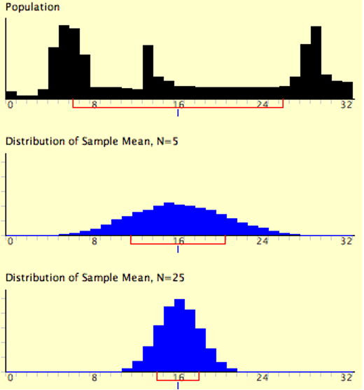
The expressions for the mean and variance of the sampling distribution of the mean are not new or remarkable. What is remarkable is that regardless of the shape of the parent population, the sampling distribution of the mean approaches a normal distribution as n increases. Figure 6.2.1 shows the results of the simulation for n = 2 and n = 10. The parent population was a uniform distribution. You can see that the distribution for n = 2 is far from a normal distribution. Nonetheless, it does show that the scores are denser in the middle than in the tails. For n = 10 the distribution is quite close to a normal distribution. Notice that the means of the two distributions are the same, but that the spread of the distribution for n = 10 is smaller.
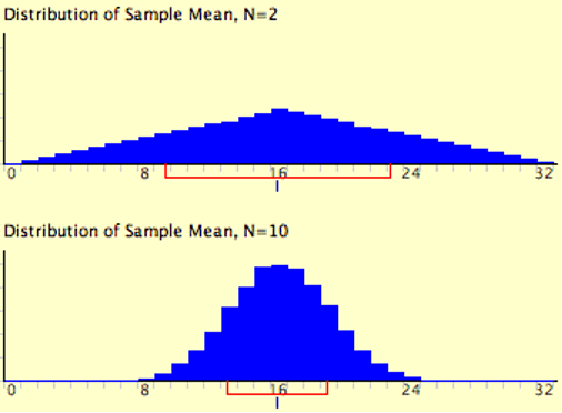
Figure 6.2.2 shows how closely the sampling distribution of the mean approximates a normal distribution even when the parent population is very non-normal. If you look closely you can see that the sampling distributions do have a slight positive skew. The larger the sample size, the closer the sampling distribution of the mean would be to a normal distribution.