Section 6.3 Calculating Confidence Intervals
Subsection 6.3.1 Confidence Intervals for the Mean
1
This subsubsection is adapted from David M. Lane. "Confidence Interval on the Mean." Online Statistics Education: A Multimedia Course of Study. https://onlinestatbook.com/2/estimation/mean.html
When you compute a confidence interval on the mean, you compute the mean of a sample in order to estimate the mean of the population. Clearly, if you already knew the population mean, there would be no need for a confidence interval. However, to explain how confidence intervals are constructed, we are going to work backwards and begin by assuming characteristics of the population. Then we will show how sample data can be used to construct a confidence interval.
Subsubsection 6.3.1.1 An Artificial Example: Using the Normal Distribution
Assume that the weights of 10-year-old children are normally distributed with a mean of 90 and a standard deviation of 36. What is the sampling distribution of the mean for a sample size of 9? Recall from Section 6.2 that the mean of the sampling distribution is \(\mu\) and the standard error of the mean is
\begin{equation*}
\sigma_{\bar{X}} = \frac{\sigma}{\sqrt{n}}
\end{equation*}
For the present example, the sampling distribution of the mean has a mean of 90 and a standard deviation of 36/3 = 12. Note that the standard deviation of a sampling distribution is its standard error. Figure 6.3.1 shows this distribution. The shaded area represents the middle 95% of the distribution and stretches from 66.48 to 113.52. These limits were computed by adding and subtracting 1.96 standard deviations to/from the mean of 90 as follows:
\begin{equation*}
90 - (1.96)(12) = 66.48
\end{equation*}
\begin{equation*}
90 + (1.96)(12) = 113.52
\end{equation*}
The value of 1.96 is based on the fact that 95% of the area of a normal distribution is within 1.96 standard deviations of the mean; 12 is the standard error of the mean given our sample size of 9.
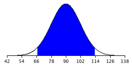
Figure 6.3.1 shows that 95% of the means are no more than 23.52 units (1.96 standard deviations) from the mean of 90. Now consider the probability that a sample mean computed in a random sample is within 23.52 units of the population mean of 90. Since 95% of the distribution is within 23.52 of 90, the probability that the mean from any given sample will be within 23.52 of 90 is 0.95. This means that if we repeatedly compute the mean (\(\bar{X}\)) from a sample (drawing a new random sample each time), and create an interval ranging from \(\bar{X} - 23.52\) to \(\bar{X} + 23.52\text{,}\) this interval will contain the population mean 95% of the time. In general, you compute the 95% confidence interval for the mean with the following formula:
\begin{gather*}
\text{Lower limit} = \bar{X} - Z_{.95}\times\sigma_{\bar{X}}\\
\text{Upper limit} = \bar{X} + Z_{.95}\times\sigma_{\bar{X}}
\end{gather*}
where \(Z_{.95}\) is the number of standard deviations extending from the mean of a normal distribution required to contain 0.95 of the area (always equal to 1.96) and \(\sigma_{\bar{X}}\) is the standard error of the mean.
If you look closely at this formula for a confidence interval, you will notice that you need to know the standard deviation (\(\sigma\)) in order to estimate the mean. This may sound unrealistic, and it is. However, computing a confidence interval when \(\sigma\) is known is easier than when \(\sigma\) has to be estimated, and serves a pedagogical purpose. Later in this section we will show how to compute a confidence interval for the mean when \(\sigma\) has to be estimated.
Suppose the following five numbers were sampled from a normal distribution with a standard deviation of 2.5: 2, 3, 5, 6, and 9. To compute the 95% confidence interval, start by computing the mean and standard error:
\begin{equation*}
\bar{X} = (2 + 3 + 5 + 6 + 9)/5 = 5.
\end{equation*}
\begin{equation*}
\sigma_{\bar{X}}=\frac{2.5}{\sqrt{5}}=1.118.
\end{equation*}
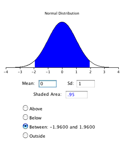
Z\(_{.95}\) can be found using the normal distribution calculator and specifying that the shaded area is 0.95 and indicating that you want the area to be between the cutoff points. As shown in Figure 6.3.2, the value is 1.96. If you had wanted to compute the 99% confidence interval, you would have set the shaded area to 0.99 and the result would have been 2.58.
The confidence interval can then be computed as follows:
\begin{gather*}
\text{Lower limit} = 5 - (1.96)(1.118)= 2.81\\
\text{Upper limit} = 5 + (1.96)(1.118)= 7.19
\end{gather*}
Subsubsection 6.3.1.2 The Realistic Case: Using the T Distribution
You should use the t distribution rather than the normal distribution when the variance is not known and has to be estimated from sample data. You will learn more about the t distribution in the next section. When the sample size is large, say 100 or above, the t distribution is very similar to the standard normal distribution. However, with smaller sample sizes, the t distribution has relatively more scores in its tails than does the normal distribution. As a result, you have to extend farther from the mean to contain a given proportion of the area. Recall that with a normal distribution, 95% of the distribution is within 1.96 standard deviations of the mean. Using the t distribution, if you have a sample size of only 5, 95% of the area is within 2.78 standard deviations of the mean. Therefore, the standard error of the mean would be multiplied by 2.78 rather than 1.96.
The values of t to be used in a confidence interval can be looked up in a table of the t distribution, a small version of which is provided in the following section. You can also use an “inverse t distribution” calculator to find the t values to use in confidence intervals. With either approach, the t values will vary depending upon the degrees of freedom (df). For confidence intervals on the mean, df is equal to n - 1, where n is the sample size.
Assume that the following five numbers are sampled from a normal distribution: 2, 3, 5, 6, and 9 and that the standard deviation is not known. The first steps are to compute the sample mean and variance:
\begin{equation*}
\bar{X} = 5
\end{equation*}
\begin{equation*}
s^2 = 7.5
\end{equation*}
The next step is to estimate the standard error of the mean. If we knew the population variance, we could use the following formula:
\begin{equation*}
\sigma_{\bar{X}} = \frac{\sigma}{\sqrt{n}}
\end{equation*}
Instead we compute an estimate of the standard error (\(s_{\bar{X}}\)). Note that since we previously computed the sample variance (\(s^2 = 7.5\)), we can take the square root of this to obtain the sample standard deviation (\(s\)):
\begin{equation*}
s_{\bar{X}} = \frac{s}{\sqrt{n}} = \frac{\sqrt{7.5}}{\sqrt{5}} = 1.225
\end{equation*}
The next step is to find the value of t. As shown in Table 6.3.5 of the following section, the value for the 95% interval for df = n - 1 = 4 is 2.776. The confidence interval is then computed just as it is when \(\sigma_{\bar{X}}\text{.}\) The only differences are that \(s_{\bar{X}}\) and \(t\) rather than \(\sigma_{\bar{X}}\) and \(Z\) are used.
\begin{gather*}
\text{Lower limit} = 5 - (2.776)(1.225) = 1.60\\
\text{Upper limit} = 5 + (2.776)(1.225) = 8.40
\end{gather*}
More generally, the formula for the 95% confidence interval on the mean is:
\begin{gather*}
\text{Lower limit} = \bar{X} - (t_{CL})(s_{\bar{X}})\\
\text{Upper limit} = \bar{X} + (t_{CL})(s_{\bar{X}})
\end{gather*}
where \(\bar{X}\) is the sample mean, \(t_{CL}\) is the t for the confidence level desired (0.95 in the above example), and \(s_{\bar{X}}\) is the estimated standard error of the mean.
We will finish our discussion of confidence intervals for the mean with an analysis of the Stroop Data. Specifically, we will compute a confidence interval on the mean difference score. As mentioned in Subsection 1.4.2, the study involved 47 subjects naming the color of ink that words were written in. An additional detail that is now relevant to us is that subjects completed similar naming tasks multiple times under different conditions. In the “interference” condition, the names conflicted so that, for example, they would name the ink color of the word “blue” written in red ink. The correct response is to say “red” and ignore the fact that the word is “blue.” In a second condition, subjects named the ink color of colored rectangles.
| Naming Colored Rectangle | Interference | Difference |
|---|---|---|
| 17 | 38 | 21 |
| 15 | 58 | 43 |
| 18 | 35 | 17 |
| 20 | 39 | 19 |
| 18 | 33 | 15 |
| 20 | 32 | 12 |
| 20 | 45 | 25 |
| 19 | 52 | 33 |
| 17 | 31 | 14 |
| 21 | 29 | 8 |
Table 6.3.3 shows the time difference between the interference and color-naming conditions for 10 of the 47 subjects. The mean time difference for all 47 subjects is 16.362 seconds and the standard deviation is 7.470 seconds. The standard error of the mean is 1.090. A t table shows the critical value of t for 47 - 1 = 46 degrees of freedom is 2.013 (for a 95% confidence interval). Therefore the confidence interval is computed as follows:
\begin{gather*}
\text{Lower limit} = 16.362 - (2.013)(1.090) = 14.17\\
\text{Upper limit} = 16.362 + (2.013)(1.090) = 18.56
\end{gather*}
Therefore, the interference effect (difference) for the whole population is likely to be between 14.17 and 18.56 seconds.
Subsection 6.3.2 More about the T Distribution
5
This section is adapted from David M. Lane. "t Distribution." Online Statistics Education: A Multimedia Course of Study. https://onlinestatbook.com/2/estimation/t_distribution.html
In the introduction to normal distributions it was shown that 95% of the area of a normal distribution is within 1.96 standard deviations of the mean. Therefore, if you randomly sampled a value from a normal distribution with a mean of 100, the probability it would be within 1.96\(\sigma\) of 100 is 0.95. Similarly, if you sample n values from the population, the probability that the sample mean (\(\bar{X}\)) will be within 1.96 \(\sigma_{\bar{X}}\) of 100 is 0.95.
Now consider the case in which you have a normal distribution but you do not know the standard deviation. You sample \(n\) values and compute the sample mean (\(\bar{X}\)) and estimate the standard error of the mean (\(\sigma_{\bar{X}}\)) with \(s_{\bar{X}}\text{.}\) What is the probability that \(\bar{X}\) will be within 1.96 \(s_{\bar{X}}\) of the population mean (\(\mu\))? This is a difficult problem because there are two ways in which \(\bar{X}\) could be more than 1.96 \(s_{\bar{X}}\) from \(\mu\text{:}\) (1) \(\bar{X}\) could, by chance, be either very high or very low and (2) \(s_{\bar{X}}\) could, by chance, be very low. Intuitively, it makes sense that the probability of being within 1.96 standard errors of the mean should be smaller than in the case when the standard deviation is known (and cannot be underestimated). But exactly how much smaller? Fortunately, the way to work out this type of problem was solved in the early 20th century by W. S. Gosset who determined the distribution of a mean divided by an estimate of its standard error. This distribution is called the Student’s t distribution or sometimes just the t distribution. Gosset worked out the t distribution and associated statistical tests while working for a brewery in Ireland. Because of a contractual agreement with the brewery, he published the article under the pseudonym “Student.” That is why the t test is called the “Student’s t test.”
The t distribution is very similar to the normal distribution when the estimate of variance is based on a large sample, but the t distribution has relatively more scores in its tails when there is a small sample. When working with the t distribution, sample size is expressed in what are called degrees of freedom. Degrees of freedom indicate the number of independent pieces of information on which an estimate is based; a more complete discussion of the concept is provided in Appendix I at the end of this chapter. As we noted in the prior section, when we are estimating the standard error for a sample mean, the degrees of freedom is simply equal to the sample size minus one (n-1).
Figure 6.3.4 shows t distributions with 2, 4, and 10 degrees of freedom and the standard normal distribution. Notice that the normal distribution has relatively more scores in the center of the distribution and the t distribution has relatively more in the tails. The t distribution approaches the normal distribution as the degrees of freedom increase.
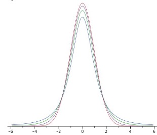
Since the t distribution has more area in the tails, the percentage of the distribution within 1.96 standard deviations of the mean is less than the 95% for the normal distribution. Table 6.3.5 shows the number of standard deviations from the mean required to contain 95% and 99% of the area of the t distribution for various degrees of freedom. These are the values of t that you use in a confidence interval. The corresponding values for the normal distribution are 1.96 and 2.58 respectively. Notice that with few degrees of freedom, the values of t are much higher than the corresponding values for a normal distribution and that the difference decreases as the degrees of freedom increase. In fact, the critical t value for probability 0.95 gets closer and closer to 1.96 (the critical value for 0.95 in the normal distribution) as the degrees of freedom increase. The values shown in Table 6.3.5 can be obtained from statistical software or an online calculator.
| df | 0.95 | 0.99 |
|---|---|---|
| 2 | 4.303 | 9.925 |
| 3 | 3.182 | 5.841 |
| 4 | 2.776 | 4.604 |
| 5 | 2.571 | 4.032 |
| 8 | 2.306 | 3.355 |
| 10 | 2.228 | 3.169 |
| 20 | 2.086 | 2.845 |
| 50 | 2.009 | 2.678 |
| 100 | 1.984 | 2.626 |
Returning to the problem posed at the beginning of this section, suppose you sampled 9 values from a normal population and estimated the standard error of the mean (\(\sigma_{\bar{X}}\)) with \(s_{\bar{X}}\text{.}\) What is the probability that \(\bar{X}\) would be within 1.96\(s_{\bar{X}}\) of \(\mu\text{?}\) Since the sample size is 9, there are n - 1 = 8 df. From Table 6.3.5, you can see that with 8 df the probability is 0.95 that the mean will be within 2.306 \(s_{\bar{X}}\) of \(\mu\text{.}\) The probability that it will be within 1.96 \(s_{\bar{X}}\) of \(\mu\) is therefore lower than 0.95.
As shown in Figure 6.3.6, a t distribution calculator can be used to find that 0.086 of the area of a t distribution is more than 1.96 standard deviations from the mean, so the probability that \(\bar{X}\) would be less than 1.96\(s_{\bar{X}}\) from \(\mu\) is 1 - 0.086 = 0.914.
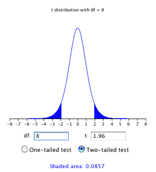
As expected, this probability is less than 0.95 that would have been obtained if \(\sigma_{\bar{X}}\) had been known instead of estimated.
Subsection 6.3.3 Confidence Intervals for a Regression Slope Coefficient
8
This section is adapted from David M. Lane. "Inferential Statistics for b and r." Online Statistics Education: A Multimedia Course of Study. https://onlinestatbook.com/2/regression/inferential.html
The method for computing a confidence interval for the population slope in a simple linear regression is very similar to methods for computing other confidence intervals. For the 95% confidence interval, the formula is:
\begin{gather*}
\text{Lower limit} = \hat{\beta} - (t_{.95})(s_{\beta})\\
\text{Upper limit} = \hat{\beta} + (t_{.95})(s_{\beta})
\end{gather*}
where \(\hat{\beta}\) is the slope coefficient estimate, \(t_{.95}\) is the value of t for 95% (2-tailed) confidence, and \(s_{\beta}\) is the standard error for the slope estimate. As before, the t value can be found from a table or an inverse t distribution calculator based on the degrees of freedom.
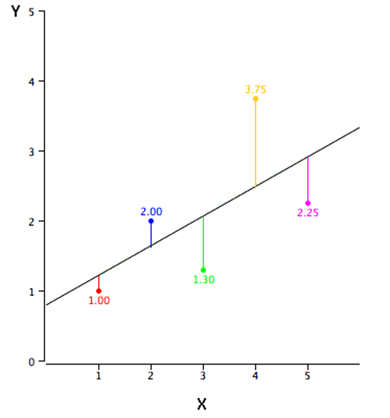
We illustrate generating a confidence interval using the same data as in the example from Section 3.4, depicted again here as Figure 6.3.7.
When conducting statistical inference for linear regression coefficients, the degrees of freedom is equal to the number of observations minus the number of coefficients being estimated (usually one for the intercept plus one for each independent variable). In the case of simple regression, there is just one independent variable plus a y-intercept, so the number of degrees of freedom is:
\begin{equation*}
df = n-2
\end{equation*}
where \(n\) is the number of pairs of scores (number of observations in the sample).
As we saw in Section 3.4, the estimated regression slope coefficient is 0.425 with this data. An \(n\) of 5 yields 3 degrees of freedom (5 - 2 = 3), which means the critical t value (at 95% confidence) is 3.182. Finally, the estimated standard error for this slope coefficient (the calculative of which is shown in this chapter’s Appendix II) is 0.305 with this data.
Applying these formulas we obtain a confidence interval with the following lower and upper limits:
\begin{gather*}
\text{Lower limit} = 0.425 - (3.182)(0.305) = -0.55\\
\text{Upper limit} = 0.425 + (3.182)(0.305) = 1.40
\end{gather*}
Subsubsection 6.3.3.1 Assumptions for Statistical Inference from Regression
Although no assumptions were needed to determine the best-fitting straight line, assumptions are made in the calculation of inferential statistics. Naturally, these assumptions refer to the population, not the sample.
-
Linearity: The relationship between the two variables is linear.
-
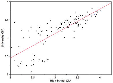
Homoscedasticity: The variance around the regression line is the same for all values of X. A clear violation of this assumption is shown in Figure 6.3.8. Notice that the predictions for students with high high-school GPAs are very good, whereas the predictions for students with low high-school GPAs are not very good. In other words, the points for students with high high-school GPAs are close to the regression line, whereas the points for low high-school GPA students are not.
-
The errors of prediction are distributed normally. This means that the deviations from the regression line are normally distributed. It does not mean that X or Y is normally distributed.
We will return to the topic of model assumptions and the consequences of violating them in Chapter 11.

