Section 8.2 Pairwise Comparisons Among Multiple Means 1
This section is adapted from David M. Lane. “All Pairwise Comparisons Among Means.” Online Statistics Education: A Multimedia Course of Study. https://onlinestatbook.com/2/tests_of_means/pairwise.html
1
This section is adapted from David M. Lane. “All Pairwise Comparisons Among Means.” Online Statistics Education: A Multimedia Course of Study. https://onlinestatbook.com/2/tests_of_means/pairwise.html
Many experiments are designed to compare more than two conditions. We will take as an example the case study “Smiles and Leniency.”In this study, the effect of different smiles on the leniency shown to a person was investigated. Four different types of smiles (neutral, false, felt, and miserable) were shown. “Type of Smile” is the independent variable, and the dependent variable is a leniency rating given by the subject to a fictional student (depicted with one of the four smiles) in an academic misconduct case. An obvious way to proceed would be to do a t test of the difference between each group mean and each of the other group means. This procedure would lead to the six comparisons shown in Table 8.4.
| false vs. felt |  |
 |
| false vs. miserable | |
 |
| false vs. neutral | |
 |
| felt vs. miserable | |
|
| felt vs. neutral | |
|
| miserable vs. neutral | |
|
The problem with this approach is that if you did this analysis, you would have six chances to make a Type I error. Therefore, if you were using the 0.05 significance level, the probability that you would make a Type I error on at least one of these comparisons is greater than 0.05. The more means that are compared, the more the Type I error rate is inflated. Figure 8.3 shows the number of possible comparisons between pairs of means (pairwise comparisons) as a function of the number of means. If there are only two means, then only one comparison can be made. If there are 12 means, then there are 66 possible comparisons.
2
When discussing probability of Type I errors, we assume all null hypotheses are true, since a Type I error can’t occur if the null hypothesis is false.
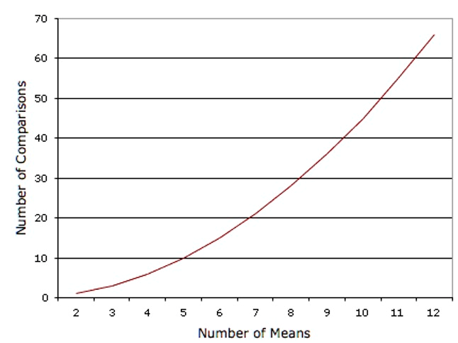
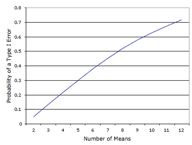
Figure 8.4shows the probability of a Type I error as a function of the number of means. As you can see, if you have an experiment with 12 means, the probability is about 0.70 that at least one of the 66 comparisons among means would be significant even if all 12 population means were the same.
The Type I error rate can be controlled using a test called the Tukey Honestly Significant Difference test or Tukey HSD for short. The Tukey HSD test is one example of a multiple comparison test, but several alternatives are frequently used, such as the Bonferroni correction. Regardless of the exact method used for a multiple comparison test, the interpretation of results is similar. The Tukey HSD is based on a variation of the t distribution that takes into account the number of means being compared. This distribution is called the studentized range distribution.
Normally, statistical software will make all the necessary calculations for you in the background. But to illustrate what sorts of calculations the software is relying on, let’s return to the leniency study to see how to compute the Tukey HSD test. You will see that the computations are very similar to those of an independent-groups t test. The steps are outlined below:
| Condition | Mean | Variance | ||||
|---|---|---|---|---|---|---|
| False | 5.37 | 3.34 | ||||
| Felt | 4.91 | 2.83 | ||||
| Miserable | 4.91 | 2.11 | ||||
| Neutral | 4.12 | 2.32 |
-
Compute MSE, which is simply the mean of the variances. It is equal to 2.65.
-
Compute Q (using the formula below) for each pair of means, where \(\bar{X}_i\) is one mean, \(\bar{X}_j\) is the other mean, and \(n\) is the number of scores in each group. For these data, there are 34 observations per group. The value in the denominator is 0.279.\begin{equation*} Q=\frac{\bar{X}_i-\bar{X}_j}{\sqrt{\frac{MSE}{n}}} \end{equation*}
-
Compute p for each comparison using a Studentized Range Calculator.The degrees of freedom is equal to the total number of observations minus the number of means. For this experiment, df = 136 - 4 = 132.
3
https://onlinestatbook.com/2/calculators/studentized_range_dist.html
| Comparison | \(\bar{X}_i - \bar{X}_j\) | \(Q\) | \(p\) |
|---|---|---|---|
| False - Felt | 0.46 | 1.65 | 0.649 |
| False - Miserable | 0.46 | 1.65 | 0.649 |
| False - Neutral | 1.25 | 4.48 | 0.010 |
| Felt - Miserable | 0.00 | 0.00 | 1.000 |
| Felt - Neutral | 0.79 | 2.83 | 0.193 |
| Miserable - Neutral | 0.79 | 2.83 | 0.193 |
The only significant comparison is between the false smile and the neutral smile.
It is not unusual to obtain results that on the surface appear paradoxical. For example, these results appear to indicate that (a) the false smile is the same as the miserable smile, (b) the miserable smile is the same as the neutral control, and (c) the false smile is different from the neutral control. This apparent contradiction is avoided if you are careful not to accept the null hypothesis when you fail to reject it. The finding that the false smile is not significantly different from the miserable smile does not mean that they are really the same. Rather it means that there is not convincing evidence that they are different. Similarly, the non-significant difference between the miserable smile and the control does not mean that they are the same. The proper conclusion is that the false smile is higher than the control and that the miserable smile is either (a) equal to the false smile, (b) equal to the control, or (c) somewhere in-between.
The assumptions of the Tukey test are essentially the same as for an independent-groups t test: normality, homogeneity of variance, and independent observations. The test is quite robust to violations of normality. Violating homogeneity of variance can be more problematical than in the two-sample case since the MSE is based on data from all groups. The assumption of independence of observations is important and should not be violated.
Subsection 8.2.1 Computer Analysis
For most computer programs, you should format your data the same way you do for an independent-groups t test. The only difference is that if you have, say, four groups, you would code each group as 1, 2, 3, or 4 rather than just 1 or 2.
Subsection 8.2.2 Tukey’s Test Need Not be a Follow-Up to ANOVA
Some textbooks introduce the Tukey test only as a follow-up to an analysis of variance (ANOVA), a technique introduced in the following section. There is no logical or statistical reason why you should not use the Tukey test even if you do not compute an ANOVA (or even know what one is). If you or your instructor do not wish to take our word for this, see the excellent article on this and other issues in statistical analysis by Leland Wilkinson and the APA Board of Scientific Affairs’ Task Force on Statistical Inference, published in theAmerican Psychologist, August 1999, Vol. 54, No. 8, 594–604.

