Section 7.5 Testing a Single Mean 1
This section is adapted from David M. Lane. "Testing a Single Mean." Online Statistics Education: A Multimedia Course of Study. https://onlinestatbook.com/2/tests_of_means/single_mean.html
1
This section is adapted from David M. Lane. "Testing a Single Mean." Online Statistics Education: A Multimedia Course of Study. https://onlinestatbook.com/2/tests_of_means/single_mean.html
The way we calculate the probability (\(p\)) value for a hypothesis test depends on what type of statement is made in our null hypothesis. Normally, statistical software will automatically compute a p value behind the scenes, but we still want to learn a bit about how the software comes up with this value. To illustrate what these calculations can look like, this section will focus on what to do if we want to test a null hypothesis stating that the population mean is equal to some hypothesized value. For example, suppose an experimenter wanted to know if people are influenced by a subliminal message and performed the following experiment. Each of nine subjects is presented with a series of 100 pairs of pictures, and for each pair they are asked to select one. As a pair of pictures is presented, a subliminal message is presented suggesting the picture that the subject should choose. The question is whether the (population) mean number of times the suggested picture is chosen is equal to 50 (the number we would expect if subliminal messages have no effect). In other words, the null hypothesis is that the population mean (\(\mu\)) is 50. The (hypothetical) data are shown in Table 7.5.1. The data in Table 7.5.1 have a sample mean (\(\bar{X}\)) of 51. Thus the sample mean differs from the hypothesized population mean by 1.
| Frequency |
|---|
| 45 |
| 48 |
| 49 |
| 49 |
| 51 |
| 52 |
| 53 |
| 55 |
| 57 |
The significance test consists of computing the probability of a sample mean differing from \(\mu\) by one (the difference between the hypothesized population mean and the sample mean) or more. The first step is to determine the sampling distribution of the mean. As we learned in the prior chapter, the mean and standard deviation of the sampling distribution of the mean are
\begin{equation*}
\mu_{\bar{X}} = \mu
\end{equation*}
and
\begin{equation*}
\sigma_{\bar{X}} = \frac{\sigma}{\sqrt{n}}
\end{equation*}
respectively. It is clear that if the null hypothesis is true, \(\mu_{\bar{X}}\) = 50. In order to compute the standard deviation of the sampling distribution of the mean, we have to know the population standard deviation (\(\sigma\)).
The current example was constructed to be one of the few instances in which the standard deviation is known. In practice, it is very unlikely that you would know \(\sigma\) and therefore you would use \(s\text{,}\) the sample estimate of \(\sigma\text{.}\) However, it is instructive to see how the probability is computed if \(\sigma\) is known before proceeding to see how it is calculated when \(\sigma\) is estimated.
For the current example, if the null hypothesis is true, then based on a well-established formula for the binomial distribution, one can compute that the variance of the number correct is
\begin{equation*}
\sigma^2 = N \pi (1-\pi) = 100(0.5)(1-0.5) = 25
\end{equation*}
where \(N\) is the number of times a subject makes a selection between two pictures. Therefore, \(\sigma\) = 5 (since \(\sigma = \sqrt{\sigma^2}=\sqrt{25}=5\)). For a \(\sigma\) of 5 and an \(n\) of 9, the standard deviation of the sampling distribution of the mean is \(5/\sqrt{9} = 1.667\text{.}\) Recall that the standard deviation of a sampling distribution is called the standard error.
To recap, we wish to know the probability of obtaining a sample mean of 51 or greater assuming the null hypothesis is true. If the null hypothesis is true, the sampling distribution of the mean has a mean of 50 and a standard deviation of 1.667. To compute the relevant probability, we will make the assumption that the sampling distribution of the mean is normally distributed. We can then use a normal distribution calculator as shown in Figure 7.5.2.
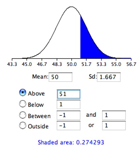
Notice that the mean is set to 50, the standard deviation to 1.667, and the area above 51 is requested and shown to be 0.274.
Therefore, the probability of obtaining a sample mean of 51 or larger is 0.274. Since a mean of 51 or higher is not unlikely under the assumption that the subliminal message has no effect, the effect is not significant and the null hypothesis is not rejected.
The test conducted above was a one-tailed test because it computed the probability of a sample mean being one or more points higher than the hypothesized mean of 50 and the area computed was the area above 51. To test the two-tailed hypothesis, you would compute the probability of a sample mean differing by one or more in either direction from the hypothesized mean of 50. You would do so by computing the probability of a mean being less than or equal to 49 or greater than or equal to 51.
The results from a normal distribution calculator are shown in Figure 7.5.3.
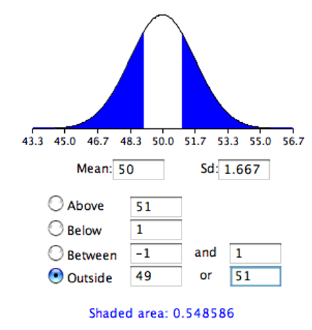
As you can see, the probability is 0.548 which, as expected, is twice the probability of 0.274 shown in Figure 7.5.2.
Before normal calculators such as the one illustrated above were widely available, probability calculations were made based on the standard normal distribution. This was done by computing \(Z\) based on the formula
\begin{equation*}
Z = \frac{\bar{X}-\mu_0}{\sigma_{\bar{X}}}
\end{equation*}
where \(Z\) is the value on the standard normal distribution, \(\bar{X}\) is the sample mean, \(\mu_0\) is the hypothesized value of the mean (under the null hypothesis), and \(\sigma_{\bar{X}}\) is the standard error of the mean. For this example, \(Z\) = (51-50)/1.667 = 0.60. Use a normal calculator, with a mean of 0 and a standard deviation of 1, as shown below.
2
The subscript \(_0\) in \(\mu_0\) (the population mean according to the null hypothesis) corresponds to how we typically represent the null hypothesis: \(H_0\text{.}\)
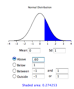
Notice that the probability (the shaded area) is the same as previously calculated (for the one-tailed test).
As noted, in real-world data analyses it is very rare that you would know \(\sigma\) and wish to estimate \(\mu\text{.}\) Typically \(\sigma\) is not known and is estimated in a sample by s, and \(\sigma_{\bar{X}}\) is estimated by \(s_{\bar{X}}\text{.}\) For our next example, we will consider the data in the “ADHD Treatment” case study. These data consist of the scores of 24 children with ADHD on a delay of gratification (DOG) task. Each child was tested under four dosage levels. Table 7.5.5 shows the data for the placebo (0 mg) and highest dosage level (0.6 mg) of methylphenidate. Of particular interest here is the column labeled “Diff” that shows the difference in performance between the 0.6 mg (D60) and the 0 mg (D0) conditions. These difference scores are positive for children who performed better in the 0.6 mg condition than in the control condition and negative for those who scored better in the control condition. If methylphenidate has a positive effect, then the mean difference score in the population will be positive. The null hypothesis is that the mean difference score in the population is 0.
| D0 | D60 | Diff |
|---|---|---|
| 57 | 62 | 5 |
| 27 | 49 | 22 |
| 32 | 30 | -2 |
| 31 | 34 | 3 |
| 34 | 38 | 4 |
| 38 | 36 | -2 |
| 71 | 77 | 6 |
| 33 | 51 | 18 |
| 34 | 45 | 11 |
| 53 | 42 | -11 |
| 36 | 43 | 7 |
| 42 | 57 | 15 |
| 26 | 36 | 10 |
| 52 | 58 | 6 |
| 36 | 35 | -1 |
| 55 | 60 | 5 |
| 36 | 33 | -3 |
| 42 | 49 | 7 |
| 36 | 33 | -3 |
| 54 | 59 | 5 |
| 34 | 35 | 1 |
| 29 | 37 | 8 |
| 33 | 45 | 12 |
| 33 | 29 | -4 |
To test this null hypothesis, we compute what we call a t statistic (as opposed to a z statistic) because we will compare this value to the t distribution—a distribution which allows for accurate inferences when \(\sigma\) is estimated rather than known (see Subsection 6.3.2). We compute t using a special case of the following formula:
\begin{equation*}
\text{t} = \frac{\text{statistic} -\text{hypothesized value}}{\text{estimated standard error of the statistic}}
\end{equation*}
The special case of this formula applicable to testing a single mean is
\begin{equation*}
\text{t} = \frac{\bar{X}-\mu_0}{s_{\bar{X}}}
\end{equation*}
where \(t\) is the value we compute for the significance test, \(\bar{X}\) is the sample mean, \(\mu_0\) is the hypothesized value of the population mean, and \(s_{\bar{X}}\) is the estimated standard error of the mean. Notice the similarity of this formula to the formula for \(Z\) we saw before.
In the previous example, we assumed that the scores were normally distributed. In this case, it is the population of difference scores that we assume to be normally distributed.
The mean (\(\bar{X}\)) of the n = 24 difference scores is 4.958, the hypothesized value of \(\mu\) is 0, and the standard deviation (s) is 7.538. The estimate of the standard error of the mean is computed as:
\begin{equation*}
s_{\bar{X}} = \frac{s}{\sqrt{n}} = \frac{7.538}{\sqrt{24}} = 1.54
\end{equation*}
Therefore, t = 4.96/1.54 = 3.22. The probability value for t depends on the degrees of freedom. The number of degrees of freedom is equal to n - 1 = 23. As shown below, a t distribution calculator finds that the probability of a t less than -3.22 or greater than 3.22 is only 0.0038. Therefore, if the drug had no effect, the probability of finding a difference between means as large or larger (in either direction) than the difference found is very low. Therefore the null hypothesis that the population mean difference score is zero can be rejected. The conclusion is that the population mean for the drug condition is higher than the population mean for the placebo condition.
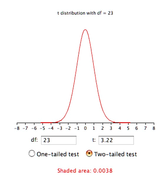
In order to conduct this hypothesis test, we made the following assumptions:
-
Each value is sampled independently from each other value.
-
The values are sampled from a normal distribution.
Now that we’ve filled in more of the details of hypothesis tests, you may want to go back and review Section 7.2 to see whether you can follow the succinct overview of the hypothesis testing approach. Once you can follow that description, it is a good indication that you have understood the key concepts essential to every hypothesis test.

