Section 8.1 Difference between Two Means 1
This section is adapted from David M. Lane. “Difference between Two Means (Independent Groups).” Online Statistics Education: A Multimedia Course of Study. https://onlinestatbook.com/2/tests_of_means/difference_means.html
1
This section is adapted from David M. Lane. “Difference between Two Means (Independent Groups).” Online Statistics Education: A Multimedia Course of Study. https://onlinestatbook.com/2/tests_of_means/difference_means.html
This section covers how to test for differences between means from two separate groups of subjects, using an independent-groups t test.
We take as an example the data from the “Animal Research” case study, previously described when discussing confidence intervals (Section 4.2.1). As a reminder, students rated (on a 7-point scale) whether they thought animal research is wrong.
| Group | n | Mean | Variance | |||||
|---|---|---|---|---|---|---|---|---|
| Females | 17 | 5.353 | 2.743 | |||||
| Males | 17 | 3.882 | 2.985 |
As we noted previously, the female mean is 1.47 units higher than the male mean (Table 8.1). This is just the difference in our sample, however, and we wish to draw an inference about the difference in the population means.
In order to test whether there is a difference between population means, we are going to make three assumptions (just as we did when constructing a confidence interval):
-
The two populations have the same variance. This assumption is called the assumption of homogeneity of variance.
-
The populations are normally distributed.
-
Each value is sampled independently. This assumption requires that each subject provide only one value. If a subject provides two scores, then the scores are not independent.
2
Two variables are said to be independent if the value of one variable provides no information about the value of the other variable. In this case, if knowing the value of the X variable for one observation could help us predict the value of X for another observation, the two values of X are not independent. For example, if there is clustered sampling, such that selecting an individual into the sample implies that neighbors with similar X values are also likely to be in the sample, the observations are not independent.
One could look at these assumptions in much more detail, but suffice it to say that small-to-moderate violations of assumptions 1 and 2 do not make much difference. It is important not to violate assumption 3.
In practice, most researchers use software to automate calculation with all formulas we encounter in this chapter. Nonetheless, your ability to understand the output of the software may improve if you have some idea of what’s happening under the hood. As we saw in the previous chapter, the following general formula is used for significance testing based on the t distribution:
\begin{equation*}
\text{t} = \frac{\text{statistic} - \text{hypothesized value}}{\text{estimated standard error of the statistic}}
\end{equation*}
In this case, our statistic is the difference between sample means and our hypothesized value is 0 because the null hypothesis states that the difference between population means is 0.
We continue to use the data from the “Animal Research” case study and will compute a significance test on the difference between the mean score of the females and the mean score of the males.
The first step is to compute the statistic, which is simply the difference between means.
\begin{equation*}
\bar{X}_1 - \bar{X}_2 = 5.3529 - 3.8824 = 1.4705
\end{equation*}
Since the hypothesized value is 0, we do not need to subtract it from the statistic.
The next step is to compute the estimate of the standard error of the statistic. In this case, the statistic is the difference between means, so the estimated standard error of the statistic is \(s_{\text{diff}}\) (which can also be written as \(s_{\bar{X}_1 - \bar{X}_2}\)). The formula for the standard error of the difference between means is:
3
For a more detailed discussion, see https://onlinestatbook.com/2/sampling_distributions/samplingdist_diff_means.html
\begin{equation*}
\sigma_{\text{diff}} = \sqrt{\frac{\sigma^2_1}{n_1}+\frac{\sigma^2_2}{n_2}} = \sqrt{\frac{\sigma^2}{n}+\frac{\sigma^2}{n}} = \sqrt{\frac{2\sigma^2}{n}}
\end{equation*}
where \(\sigma^2_1\) and \(n_1\) are the variance and sample size of the first group, and \(\sigma^2_2\) and \(n_2\) are the variance and sample size of the second group. Note that since we assumed \(\sigma^2_1 = \sigma^2_2\) (as our first of the three assumptions listed above), we can represent both of these variances as simply \(\sigma^2\text{.}\) Likewise, when \(n_1\) = \(n_2\) (as in our example with equal numbers of females and males), it is conventional to use “\(n\)” to refer to the sample size of each group.
Because the value of \(\sigma^2\) is unknown, we estimate it by averaging our two sample variances, relying again on our assumption that the two population variances are the same (and thus each sample’s variance should be an equally valid estimate of \(\sigma^2\)). This estimate of variance is can be written as follows:
\begin{equation*}
\text{MSE}= \frac{s^2_1+s^2_2}{2}
\end{equation*}
where MSE is our estimate of \(\sigma^2\text{.}\) In this example,
\begin{equation*}
\text{MSE} = (2.743 + 2.985)/2 = 2.864.
\end{equation*}
We can now estimate \(\sigma_{\text{diff}}\) with \(s_{\text{diff}}\text{,}\) substituting in MSE where we previously saw \(\sigma^2\) in the formula for \(\sigma_{\text{diff}}\text{.}\) Since n (the number of scores in each group) is 17,
\begin{equation*}
s_{\text{diff}} = \sqrt{\frac{2MSE}{n}} = \sqrt{\frac{(2)(2.864)}{17}} = 0.5805.
\end{equation*}
The next step is to compute t by plugging these values into the formula:
\begin{equation*}
t = \frac{1.4705}{0.5805} = 2.533.
\end{equation*}
Finally, we compute the probability of getting a \(t\) as large or larger than 2.533 or as small or smaller than -2.533. To do this, we need to know the degrees of freedom. The degrees of freedom is the number of independent estimates of variance on which \(MSE\) is based. This is equal to (\(n_1\)- 1) + (\(n_2\)- 1), and for this example,\(n_1\) = \(n_2\)= 17. Therefore, the degrees of freedom is 16 + 16 = 32.
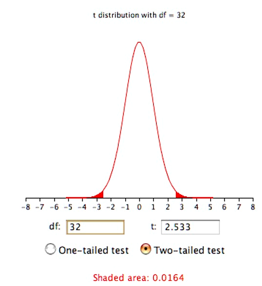
Once we have the degrees of freedom, we can use a t distribution calculator to find the probability. Figure 8.1 shows that the probability value (p) for a two-tailed test is 0.0164. The two-tailed test is used when the null hypothesis can be rejected regardless of the direction of the effect. As shown in Figure 8.1, it is the probability of a t < -2.533 or a t > 2.533.
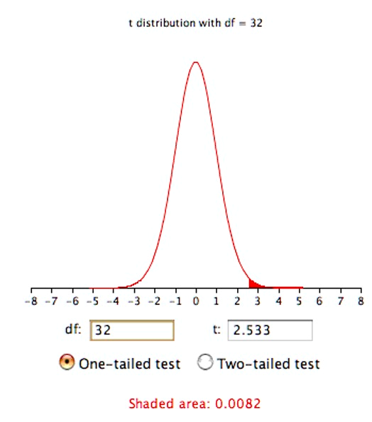
The results of a one-tailed test are shown in Figure 8.2. As you can see, the probability value of 0.0082 is half the value for the two-tailed test.
Subsection 8.1.1 Formatting Data for Computer Analysis
Most computer programs that compute t tests require your data to be in a specific form. Consider the data in Table 8.2.
| Group 1 | Group 2 | |||
|---|---|---|---|---|
| 3 | 2 | |||
| 4 | 6 | |||
| 5 | 8 |
Here there are two groups, each with three observations. To format these data for a computer program, you normally have to use two variables: the first specifies the group the subject is in and the second is the score itself. The reformatted version of the data in Table 8.2 is shown in Table 8.3. We sometimes describe the original format as “wide” form and the reformatted data as “long” form.
| Group | Y | |||
|---|---|---|---|---|
| 1 | 3 | |||
| 1 | 4 | |||
| 1 | 5 | |||
| 2 | 2 | |||
| 2 | 6 | |||
| 2 | 8 |
Using statistical software, we’d find that the t value is -0.718, the df = 4, and p = 0.512.

