Section 3.4 Introduction to Linear Regression
1
This section is adapted from David M. Lane. "Introduction to Linear Regression." Online Statistics Education: A Multimedia Course of Study. https://onlinestatbook.com/2/regression/intro.html
In simple linear regression, we predict scores on one variable from the scores on a second variable. The variable we are predicting is called the dependent variable and is referred to as \(Y\text{.}\) The variable we are basing our predictions on is called the independent variable and is referred to as \(X\text{.}\) When there is only one predictor variable, the prediction method is called simple regression. In simple linear regression, the topic of this section, the predictions of \(Y\) when plotted as a function of \(X\) form a straight line.
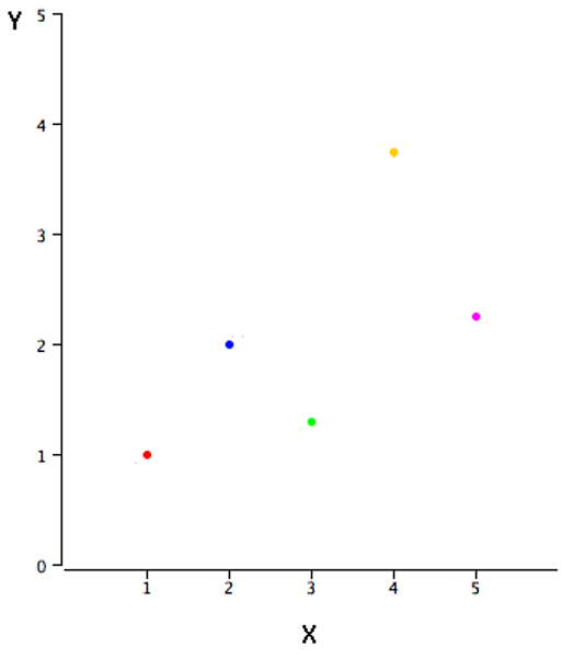
The example data in Table 3.4.1 are plotted in Figure 3.4.2. You can see that there is a positive relationship between \(X\) and \(Y\text{.}\) If you were going to predict \(Y\) from \(X\text{,}\) the higher the value of \(X\text{,}\) the higher your prediction of \(Y\text{.}\)
| \(X\) | \(Y\) |
|---|---|
| 1.00 | 1.00 |
| 2.00 | 2.00 |
| 3.00 | 1.30 |
| 4.00 | 3.75 |
| 5.00 | 2.25 |
Linear regression consists of finding the best-fitting straight line through the points. The best-fitting line is called a regression line. The black diagonal line in Figure 3.4.3 is the regression line and consists of the predicted score on \(Y\) for each possible value of \(X\text{.}\) The vertical lines from the points to the regression line represent the errors of prediction. As you can see, the red point is very near the regression line; its error of prediction is small. By contrast, the yellow point is much higher than the regression line and therefore its error of prediction is large.
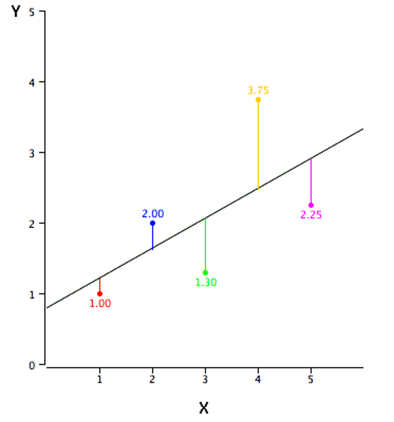
The error of prediction for a point is the value of the point minus the predicted value (the value on the line). Table 3.4.4 shows the predicted values (\(\hat{Y}\)) and the errors of prediction (\(Y - \hat{Y}\)). For example, the first point has a \(Y\) of 1.00 and a predicted \(Y\) (called \(\hat{Y}\)) of 1.21. Therefore, its error of prediction is -0.21.
| \(X\) | \(Y\) | \(\hat{Y}\) | \(Y - \hat{Y}\) | \((Y - \hat{Y})^2\) |
|---|---|---|---|---|
| 1.00 | 1.00 | 1.210 | -0.210 | 0.044 |
| 2.00 | 2.00 | 1.635 | 0.365 | 0.133 |
| 3.00 | 1.30 | 2.060 | -0.760 | 0.578 |
| 4.00 | 3.75 | 2.485 | 1.265 | 1.600 |
| 5.00 | 2.25 | 2.910 | -0.660 | 0.436 |
You may have noticed that we did not specify what is meant by “best-fitting line.” By far, the most commonly-used criterion for the best-fitting line is the line that minimizes the sum of the squared errors of prediction. That is the criterion that was used to find the line in Figure 3.4.3. The last column in Table 3.4.4 shows the squared errors of prediction. The sum of the squared errors of prediction shown in Table 3.4.4 is lower than it would be for any other regression line.
The formula for a regression line is
\begin{equation*}
\hat{Y} = \alpha + \beta X
\end{equation*}
where \(\hat{Y}\) is the predicted score, \(\alpha\) is the \(Y\)-intercept, and \(\beta\) is the slope of the line. The equation for the line in Figure 3.4.3 is
\begin{equation*}
\hat{Y} = 0.785 + 0.425X
\end{equation*}
Using this equation, we can calculate predictions for \(Y\) based on the value of \(X\text{.}\) For \(X = 1\text{,}\)
\begin{equation*}
\hat{Y} = 0.785 + (0.425)(1) = 1.21
\end{equation*}
For \(X = 2\text{,}\)
\begin{equation*}
\hat{Y} = 0.785 + (0.425)(2) = 1.64
\end{equation*}
Subsection 3.4.1 A Real Example
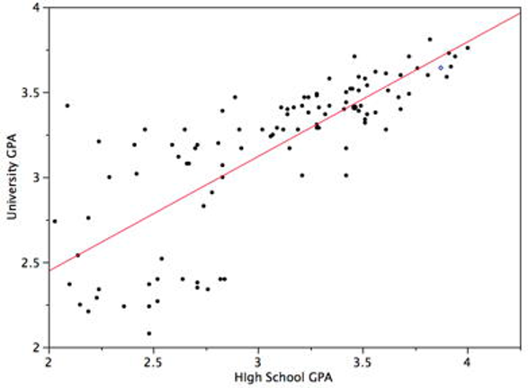
The case study “SAT and College GPA” contains high school and university grades for 105 computer science majors at a local state school. We now consider how we could predict a student’s university GPA if we knew his or her high school GPA.
Figure 3.4.5 shows a scatter plot of University GPA as a function of High School GPA. You can see from the figure that there is a strong positive relationship. The correlation is 0.78. The regression equation is
\begin{equation*}
\widehat{\text{University GPA}} = (0.675)(\text{High School GPA}) + 1.097
\end{equation*}
Therefore, a student with a high school GPA of 3 would be predicted to have a university GPA of
\begin{equation*}
\widehat{\text{University GPA}} = (0.675)(3) + 1.097 = 3.12
\end{equation*}