Section 5.2 Normal Distributions
1
The initial part of this section is adapted from David M. Lane. "Introduction to Normal Distributions." Online Statistics Education: A Multimedia Course of Study. https://onlinestatbook.com/2/normal_distribution/intro.html
The normal distribution is the most important and most widely used distribution in statistics. It is sometimes called the “bell curve,” although the tonal qualities of such a bell would be less than pleasing. It is also called the “Gaussian curve” after the mathematician Karl Friedrich Gauss. Although Gauss played an important role in its history, Abraham de Moivre first discovered the normal distribution.
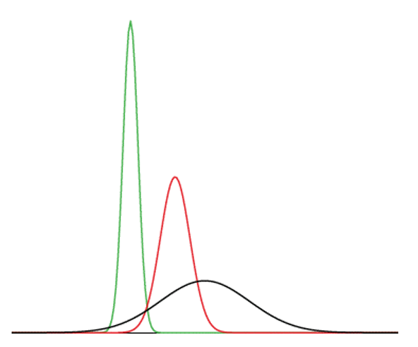
Strictly speaking, it is not correct to talk about “the normal distribution” since there are many normal distributions. Normal distributions can differ in their means and in their standard deviations. Figure 5.2.1 shows three normal distributions. The green (left-most) distribution has a mean of -3 and a standard deviation of 0.5, the distribution in red (the middle distribution) has a mean of 0 and a standard deviation of 1, and the distribution in black (right-most) has a mean of 2 and a standard deviation of 3. These as well as all other normal distributions are symmetric with relatively more values at the center of the distribution and relatively few in the tails.
Seven features of normal distributions are listed below. Some of these features are illustrated in more detail in the remaining sections of this chapter.
-
Normal distributions are symmetric around their mean.
-
The mean, median, and mode of a normal distribution are equal.
-
The area under the normal curve is equal to 1.0.
-
Normal distributions are denser in the center and less dense in the tails.
-
Normal distributions are defined by two parameters, the mean (\(\mu\)) and the standard deviation (\(\sigma\)).
-
68% of the area of a normal distribution is within one standard deviation of the mean.
-
Approximately 95% of the area of a normal distribution is within two standard deviations of the mean.
Subsection 5.2.1 Importance of Normal Distributions
2
This subsection is adapted from David M. Lane. "History of the Normal Distribution." Online Statistics Education: A Multimedia Course of Study. https://onlinestatbook.com/2/normal_distribution/history_normal.html
The importance of the normal curve stems primarily from the fact that the distributions of many natural phenomena are at least approximately normally distributed. One of the first applications of the normal distribution was to the analysis of errors of measurement made in astronomical observations, errors that occurred because of imperfect instruments and imperfect observers. Galileo in the 17th century noted that these errors were symmetric and that small errors occurred more frequently than large errors. This led to several hypothesized distributions of errors, but it was not until the early 19th century that it was discovered that these errors followed a normal distribution. Independently, the mathematicians Adrain in 1808 and Gauss in 1809 developed the formula for the normal distribution and showed that errors were fit well by this distribution.
Most statistical procedures for testing differences between means assume normal distributions. Because the distribution of means is very close to normal, these tests work well even if the original distribution is only roughly normal.
Quételet was the first to apply the normal distribution to human characteristics. He noted that characteristics such as height, weight, and strength were normally distributed.
Subsection 5.2.2 Areas Under Normal Distributions
3
This subsection is adapted from David M. Lane. "Areas Under Normal Distributions." Online Statistics Education: A Multimedia Course of Study. https://onlinestatbook.com/2/normal_distribution/areas_normal.html
Areas under portions of a normal distribution can be computed by using calculus. Since this is a non-mathematical treatment of statistics, we will rely on computer programs and tables to determine these areas.
Figure 5.2.2 shows a normal distribution with a mean of 50 and a standard deviation of 10. The shaded area between 40 and 60 contains 68% of the distribution.
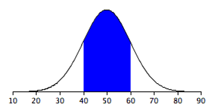
Figure 5.2.3 shows a normal distribution with a mean of 100 and a standard deviation of 20. As in Figure 5.2.2, 68% of the distribution is within one standard deviation of the mean.
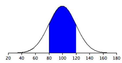
The normal distributions shown in Figure 5.2.2 and Figure 5.2.3 are specific examples of the general rule that 68% of the area of any normal distribution is within one standard deviation of the mean.
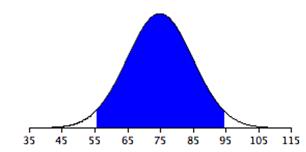
Figure 5.2.4 shows a normal distribution with a mean of 75 and a standard deviation of 10. The shaded area contains 95% of the area and extends from 55.4 to 94.6. For all normal distributions, 95% of the area is within 1.96 standard deviations of the mean. For quick approximations, it is sometimes useful to round off and use 2 rather than 1.96 as the number of standard deviations you need to extend from the mean so as to include 95% of the area.
It is easy to find free online normal distribution calculators that will give you the areas under the normal distribution (e.g.,
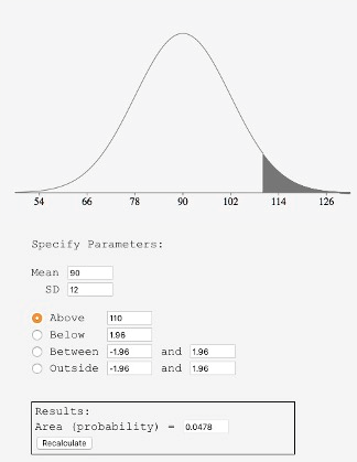
https://onlinestatbook.com/2/calculators/normal_dist.html). For example, you can use one to find the proportion of a normal distribution with a mean of 90 and a standard deviation of 12 that is above 110 (Figure 5.2.5). Set the mean to 90 and the standard deviation to 12. Then enter “110” in the box to the right of the radio button “Above.” At the bottom of the display you will see that the shaded area is 0.0478. See if you can use the calculator to find that the area between 115 and 120 is 0.0124.
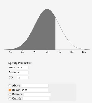
Say you wanted to find the score corresponding to the 75th percentile of a normal distribution with a mean of 90 and a standard deviation of 12. Using an inverse normal calculator (e.g.,
https://onlinestatbook.com/2/calculators/inverse_normal_dist.html), you enter the parameters as shown in Figure 5.2.6 and find that the area below 98.09 is 0.75.
Subsection 5.2.3 The Standard Normal Distribution
4
This subsection is adapted from David M. Lane. "Standard Normal Distribution." Online Statistics Education: A Multimedia Course of Study. https://onlinestatbook.com/2/normal_distribution/standard_normal.html
As discussed above, normal distributions do not necessarily have the same means and standard deviations. A normal distribution with a mean of 0 and a standard deviation of 1 is called a standard normal distribution.
A value from any normal distribution can be transformed into its corresponding value on a standard normal distribution using the following formula:
\begin{equation*}
Z = \frac{X - \mu}{\sigma}
\end{equation*}
where \(Z\) is the value on the standard normal distribution, \(X\) is the value on the original distribution, \(\mu\) is the mean of the original distribution, and \(\sigma\) is the standard deviation of the original distribution. Note that this transformation is one we already learned about (“standardization”) in Subsection 2.4.1. Here, we are highlighting that this transformation can be used to relate any normal distribution to the standard normal distribution.

