Section 2.4 Transforming Variables
1
The initial part of this section is adapted from David M. Lane. "Linear Transformations." Online Statistics Education: A Multimedia Course of Study.
https://onlinestatbook.com/2/introduction/linear_transforms.html. There is also material adapted from David M. Lane. "Standard Normal Distribution." Online Statistics Education: A Multimedia Course of Study. https://onlinestatbook.com/2/normal_distribution/standard_normal.html.
Often it is necessary to transform data from one measurement scale to another. For example, you might want to convert height measured in feet to height measured in inches. Table 2.4.1 shows the heights of four people measured in both feet and inches. To transform feet to inches, you simply multiply by 12. Similarly, to transform inches to feet, you divide by 12.
| Feet | Inches |
|---|---|
| 5.00 | 60 |
| 6.25 | 75 |
| 5.50 | 66 |
| 5.75 | 69 |
Some conversions require that you multiply by a number and then add a second number. A good example of this is the transformation between degrees Centigrade and degrees Fahrenheit. Table 2.4.2 shows the temperatures of 5 US cities in the early afternoon of November 16, 2002.
| City | Degrees Fahrenheit | Degrees Centigrade |
|---|---|---|
| Houston | 54 | 12.22 |
| Chicago | 37 | 2.78 |
| Minneapolis | 31 | -0.56 |
| Miami | 78 | 25.56 |
| Phoenix | 70 | 21.11 |
The formula to transform Centigrade to Fahrenheit is:
\begin{equation*}
F = 1.8C + 32
\end{equation*}
The formula for converting from Fahrenheit to Centigrade is
\begin{equation*}
C = 0.5556F - 17.778
\end{equation*}
The transformation consists of multiplying by a constant and then adding a second constant. For the conversion from Centigrade to Fahrenheit, the first constant is 1.8 and the second is 32.
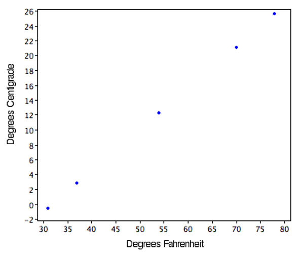
Figure 2.4.3 shows a plot of degrees Centigrade as a function of degrees Fahrenheit. Notice that the points form a straight line. This will always be the case if the transformation from one scale to another consists of multiplying by one constant and then adding a second constant. Such transformations are therefore called linear transformations.
Subsection 2.4.1 Standardization (Z Scores)
So far, we’ve discussed transformations that are probably familiar to you. A type of transformation that may be new to you is standardization or creating \(Z\) scores. A value from any distribution can be transformed into a \(Z\) score using the following formula:
\begin{equation*}
Z = \frac{(X - \mu)}{\sigma}
\end{equation*}
where \(Z\) is the new value, \(X\) is the value on the original distribution, \(\mu\) is the mean of the original distribution, and \(\sigma\) is the standard deviation of the original distribution.
As a simple application, suppose you want the \(Z\) score for a value of 26 taken from a distribution with a mean of 50 and a standard deviation of 10. Applying the formula, we obtain:
\begin{equation*}
Z = (26 - 50)/10 = -2.4
\end{equation*}
If all the values in a distribution are transformed to \(Z\) scores, then the new distribution will have a mean of 0 and a standard deviation of 1. This process of transforming a distribution to one with a mean of 0 and a standard deviation of 1 is called standardizing the distribution. Sometimes it will be easier to work with a standardized version of a variable.
Subsection 2.4.2 Log Transformations
2
This subsection is adapted from David M. Lane. "Log Transformations." Online Statistics Education: A Multimedia Course of Study.
https://onlinestatbook.com/2/transformations/log.html
Sometimes it is also useful to use transformations that are not linear. For example, the log transformation can be used to make highly skewed distributions less skewed. This can be valuable both for making patterns in the data more interpretable and for helping to meet the assumptions of inferential statistics (see Chapter 4 4).
Figure 2.4.4 shows an example of how a log transformation can make patterns more visible. Both graphs plot the brain weight of animals as a function of their body weight. The raw weights are shown in the upper panel; the log-transformed weights are plotted in the lower panel.
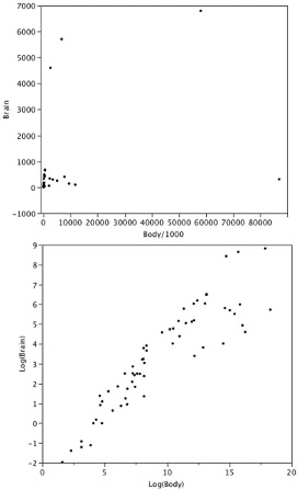
It is hard to discern a pattern in the upper panel whereas the strong relationship is shown clearly in the lower panel.

