Statistics Minus the Maths

I now move beyond the gender binary and consider the “other” category in survey responses. I’ll refer to this other category as “non-binary” gender, although the data was collected at a time when survey items were not generally designed with this group in mind; thus, we might expect that this “other” category is only a rough proxy for a non-binary gender identity. The average level of extroversion among those with non-binary gender is -5.66. So people in this dataset identified as likely non-binary tend to be quite a bit more introverted than those who identify as male or female. As with males and females, there is still considerable variation among non-binary people (Figure 12.2.1).

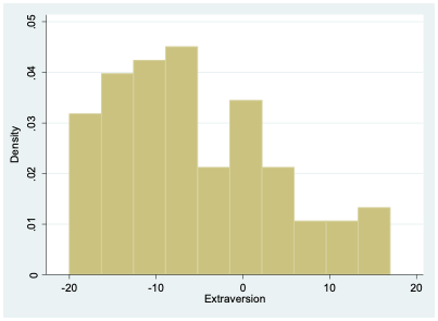
The number of non-binary respondents is relatively small (102), so it’s not terribly surprising that this histogram looks a bit choppier than the ones we saw before.

Again, if we had to make a guess about the level of extroversion of someone, and all we knew about that person was that their gender was non-binary, we would probably want to guess the mean value among non-binary respondents (-5.66). Modifying (12.1.1) to incorporate a third category is relatively straightforward:

For someone who identifies as female, we would plug in Female = 1, Male = 0, and Other = 0:

If someone identifies as non-binary, we would use Female = 0, Male = 0, and Other = 1:

We can also return to the format of (12.1.2) but modify it to include the other category. This is how we will typically write our equation if we are doing a regression:

Now that there are three possible values for gender (female, male, and other), knowing the value of Male doesn’t necessarily allow us to conclude what the value of female is. If Male = 0, the individual could identify as either female or non-binary. So we have to include a second variable. In this case, we chose to include the variable Other. If we know the values of Male and Other, we can always figure out the value of Female by process of elimination.

For a non-binary person, we plug in Male = 0, and Other = 1:

When considering a female, we use Male = 0, and Other = 0:

(12.2.1) and (12.2.2) communicate an equivalent method of making a prediction about extroversion based on gender; they just offer this information in two different formats. (12.2.2) might be a bit trickier to understand for now, but it will become very useful in the future.

Notice that we can talk about gender either as one qualitative variable with three possible values (female, male, or other), or we can talk about it as a series of three variables (Female, Male, and Other) that can take each on a value of either 0 or 1 (we call such variables “binary” or “dummy” variables). This can make things a bit confusing, but the important thing to remember is that when we have a qualitative variable with more than two categories, we’ll need to break out the categories into a set of dummy variables for purposes of representing the qualitative variable in an equation.

However, as (12.1.2) and (12.2.2) illustrate, we don’t necessarily need a dummy variable for every single category. Specifically, whenever we want to create an equation with a qualitative independent variable in a format like (12.1.2) or (12.2.2), the number of dummy variables should be equal to the number of categories minus one. Since our gender variable can take on three possible values in this example, we included two independent variables in (12.2.2). No dummy variable is included for female, so we call female the omitted category, also known as the reference group or baseline category. Remember, the first number in (12.2.2) is 0.53, which represents our guess for females—the baseline category. If we instead had a qualitative variable with five categories, we would include four dummy variables in our equation.

As we will see at the end of the next chapter, it doesn’t really matter which group we select as the omitted category because we get equivalent predictions regardless of which one we choose.