Section 2.3 Measures of Spread
1
This section is adapted from David M. Lane. "Measures of Variability." Online Statistics Education: A Multimedia Course of Study.
https://onlinestatbook.com/2/summarizing_distributions/variability.html
Subsection 2.3.1 What is Variability?
Variability refers to how “spread out” a group of scores is. To see what we mean by spread out, consider graphs in Figure 2.3.1. These graphs represent the scores on two quizzes. The mean score for each quiz is 7.0. Despite the equality of means, you can see that the distributions are quite different. Specifically, the scores on Quiz 1 are more densely packed and those on Quiz 2 are more spread out. The differences among students were much greater on Quiz 2 than on Quiz 1.
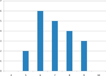
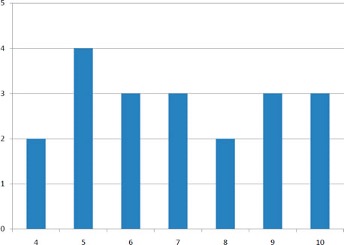
The terms variability, spread, and dispersion are synonyms, and refer to how spread out a distribution is. Just as in the section on central tendency where we discussed measures of the center of a distribution of scores, in this section we will discuss measures of the variability of a distribution. There are four frequently used measures of variability: the range, interquartile range, variance, and standard deviation. In the next few paragraphs, we will look at each of these four measures of variability in more detail.
Subsection 2.3.2 Range
The range is the simplest measure of variability to calculate, and one you have probably encountered many times in your life. The range is simply the highest score minus the lowest score. Let’s take a few examples. What is the range of the following group of numbers: 10, 2, 5, 6, 7, 3, 4? Well, the highest number is 10, and the lowest number is 2, so 10 - 2 = 8. The range is 8. Let’s take another example. Here’s a dataset with 10 numbers: 99, 45, 23, 67, 45, 91, 82, 78, 62, 51. What is the range? The highest number is 99 and the lowest number is 23, so 99 - 23 equals 76; the range is 76. Now consider the two quizzes shown in Figure 2.3.1. On Quiz 1, the lowest score is 5 and the highest score is 9. Therefore, the range is 4. The range on Quiz 2 was larger: the lowest score was 4 and the highest score was 10. Therefore the range is 6.
Subsection 2.3.3 Interquartile Range
The interquartile range (IQR) is the range of the middle 50% of the scores in a distribution. It is computed as follows:
\begin{equation*}
IQR = \text{ 75th percentile } - \text{ 25th percentile }
\end{equation*}
For Quiz 1, the 75th percentile is 8 and the 25th percentile is 6. The interquartile range is therefore 2. For Quiz 2, which has greater spread, the 75th percentile is 9, the 25th percentile is 5, and the interquartile range is 4. Recall that in the discussion of box plots (Section 1.4.2 1.4.2), the 75th percentile was called the upper hinge and the 25th percentile was called the lower hinge. Thus, the interquartile range is neatly depicted by the box portion of a boxplot.
Subsection 2.3.4 Variance
Variability can also be defined in terms of how close the scores in the distribution are to the middle of the distribution. Using the mean as the measure of the middle of the distribution, the variance is defined as the average squared difference of the scores from the mean. The data from Quiz 1 are shown in Table 2.3.2. The mean score is 7.0. Therefore, the column “Deviation from Mean” contains the score minus 7. The column “Squared Deviation” is simply the previous column squared.
| Scores | Deviation from Mean | Squared Deviation |
|---|---|---|
| Means | ||
| 9 | 2 | 4 |
| 9 | 2 | 4 |
| 9 | 2 | 4 |
| 8 | 1 | 1 |
| 8 | 1 | 1 |
| 8 | 1 | 1 |
| 8 | 1 | 1 |
| 7 | 0 | 0 |
| 7 | 0 | 0 |
| 7 | 0 | 0 |
| 7 | 0 | 0 |
| 7 | 0 | 0 |
| 6 | -1 | 1 |
| 6 | -1 | 1 |
| 6 | -1 | 1 |
| 6 | -1 | 1 |
| 6 | -1 | 1 |
| 5 | -2 | 4 |
| 5 | -2 | 4 |
| 7 | 0 | 1.5 |
One thing that is important to notice is that the mean deviation from the mean is 0. This will always be the case. The mean of the squared deviations is 1.5. Therefore, the variance is 1.5. Analogous calculations with Quiz 2 show that its variance is 6.7. The formula for the variance is:
\begin{equation*}
\sigma^2=\frac{\sum (X-\mu)^2}{N}
\end{equation*}
where \(\sigma^2\) is the variance, \(\mu\) is the mean, and \(N\) is the number of numbers. For Quiz 1, \(\mu\) = 7 and \(N\) = 20.
If the variance in a sample is used to estimate the variance in a population, then the previous formula underestimates the variance and the following formula should be used:
\begin{equation*}
s^2=\frac{\sum(X-\bar{X})^2}{n-1}
\end{equation*}
Note that \(\bar{X}\) is the mean of a sample taken from a population with a mean of \(\mu\text{.}\) Since, in practice, the variance is usually computed in a sample, this formula is most often used. While it is not easy to succinctly explain why we divide by \(n-1\) rather than simply \(n\text{,}\) the simulation “estimating variance” illustrates the bias that arises if we use \(n\) as the denominator in the formula.
Let’s look at a concrete example of calculating the sample variance. Assume the scores 1, 2, 4, and 5 were sampled from a larger population. To estimate the variance in the population you would compute \(s^2\) as follows:
\begin{equation*}
\bar{X} = (1 + 2 + 4 + 5)/4 = 12/4 = 3
\end{equation*}
\begin{align*}
s^2 \amp = [(1-3)^2 + (2-3)^2 + (4-3)^2 + (5-3)^2]/(4-1)\\
\amp = (4 + 1 + 1 + 4)/3 = 10/3 = 3.333
\end{align*}
Subsection 2.3.5 Standard Deviation
The standard deviation is simply the square root of the variance. This makes the standard deviations of the two quiz distributions 1.225 and 2.588. We can interpret the standard deviation of X as approximating the typical distance between a given value of X and the mean of X. For example, suppose I tell you about a prison where the prisoners have a mean age of 42 years with a standard deviation of 8 years. If I randomly select one prisoner and ask you to guess their age, you should probably guess 42 since I’ve told you that is the mean. But even though 42 is your best guess, you can expect your guess to be off by about 8 years since the standard deviation is 8 (meaning the typical distance between a random prisoner’s age and the mean age is approximately 8). You can’t say ahead of time which direction your guess is likely to be off (guessing too old versus too young), just that you are likely to miss the reality for a randomly-selected individual by about 8 years on a typical guess (though any one guess may happen to be closer or further than 8 years).

