Chapter 2 Basics
R Markdown provides an authoring framework for data science. You can use a single R Markdown file to both
-
save and execute code, and
-
generate high quality reports that can be shared with an audience.
R Markdown was designed for easier reproducibility, since both the computing code and narratives are in the same document, and results are automatically generated from the source code. R Markdown supports dozens of static and dynamic/interactive output formats.
If you prefer a video introduction to R Markdown, we recommend that you check out the website https://rmarkdown.rstudio.com and watch the videos in the "Get Started" section, which cover the basics of R Markdown.
Below is a minimal R Markdown document, which should be a plain-text file, with the conventional extension
.Rmd:
---
title: "Hello R Markdown"
author: "Awesome Me"
date: "2018-02-14"
output: html_document
---
This is a paragraph in an R Markdown document.
Below is a code chunk:
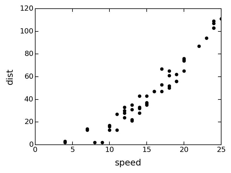
```{r}
fit = lm(dist ~ speed, data = cars)
b = coef(fit)
plot(cars)
abline(fit)
```
The slope of the regression is `r b[1]`.
You can create such a text file with any editor (including but not limited to RStudio). If you use RStudio, you can create a new Rmd file from the menu
File -> New File -> R Markdown.
There are three basic components of an R Markdown document: the metadata, text, and code. The metadata is written between the pair of three dashes
---. The syntax for the metadata is YAML (YAML Ain’t Markup Language, https://en.wikipedia.org/wiki/YAML), so sometimes it is also called the YAML metadata or the YAML frontmatter. Before it bites you hard, we want to warn you in advance that indentation matters in YAML, so do not forget to indent the sub-fields of a top field properly. See the Appendix B.2 of [6] for a few simple examples that show the YAML syntax.
The body of a document follows the metadata. The syntax for text (also known as prose or narratives) is Markdown, which is introduced in Section 2.5. There are two types of computer code, which are explained in detail in Section 2.6:
-
A code chunk starts with three backticks like
```{r}whererindicates the language name,and ends with three backticks. You can write chunk options in the curly braces (e.g., set the figure height to 5 inches:1
It is not limited to the R language; see Section 2.7 for how to use other languages.```{r, fig.height=5}).
Figure 2.1 shows the above example in the RStudio IDE. You can click the
Knit button to compile the document (to an HTML page). Figure 2.2 shows the output in the RStudio Viewer.
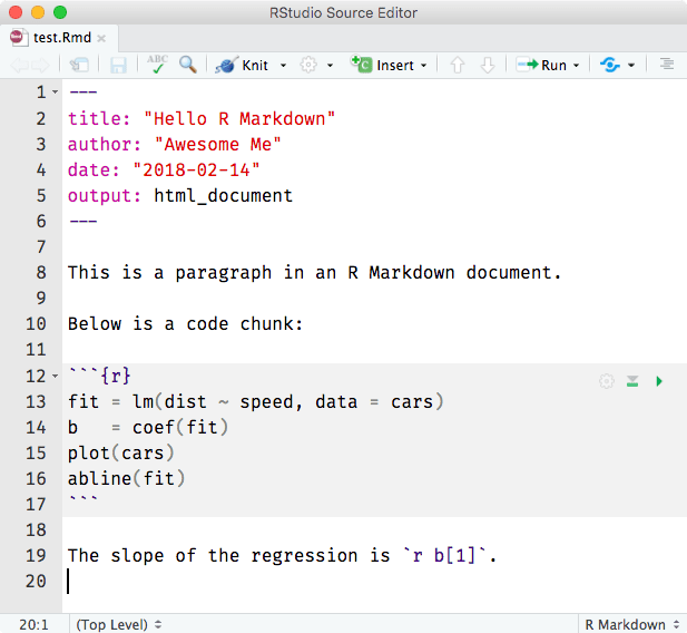
A minimal R Markdown example in RStudio.
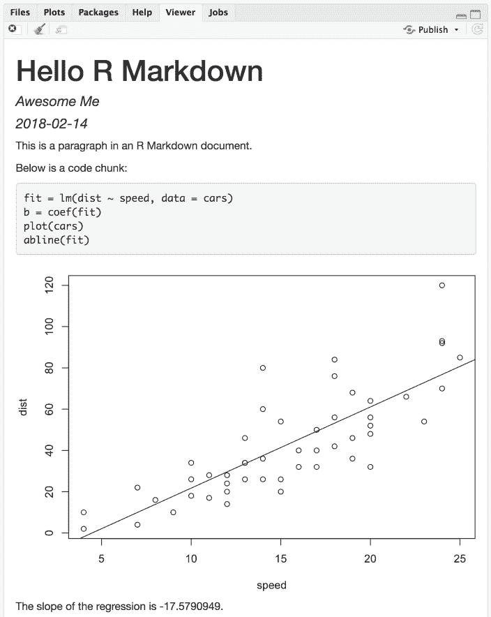
The output document of the minimal R Markdown example in RStudio.
Now please take a closer look at the example. Did you notice a problem? The object
b is the vector of coefficients of length 2 from the linear regression; b[1] is actually the intercept, and b[2] is the slope! This minimal example shows you why R Markdown is great for reproducible research: it includes the source code right inside the document, which makes it easy to discover and fix problems, as well as update the output document. All you have to do is change b[1] to b[2], and click the Knit button again. Had you copied a number -17.579 computed elsewhere into this document, it would be very difficult to realize the problem. In fact, I had used this example a few times by myself in my presentations before I discovered this problem during one of my talks, but I discovered it anyway.
Although the above is a toy example, it could become a horror story if it happens in scientific research that was not done in a reproducible way (e.g., cut-and-paste). Here are two of my personal favorite videos on this topic:
-
"A reproducible workflow" by Ignasi Bartomeus and Francisco Rodríguez-Sánchez (
https://youtu.be/s3JldKoA0zwIt is a 2-min video that looks artistic but also shows very common and practical problems in data analysis.
-
"The Importance of Reproducible Research in High-Throughput Biology" by Keith Baggerly (
https://youtu.be/7gYIs7uYbMoYou will be impressed by both the content and the style of this lecture. Keith Baggerly and Kevin Coombes were the two notable heroes in revealing the Duke/Potti scandal, which was described as "one of the biggest medical research frauds ever" by the television program "60 Minutes".
It is fine for humans to err (in computing), as long as the source code is readily available.
Section 2.1 Example applications
Now you have learned the very basic concepts of R Markdown. The idea should be simple enough: interweave narratives with code in a document, knit the document to dynamically generate results from the code, and you will get a report. This idea was not invented by R Markdown, but came from an early programming paradigm called "Literate Programming" [3].
Due to the simplicity of Markdown and the powerful R language for data analysis, R Markdown has been widely used in many areas. Before we dive into the technical details, we want to show some examples to give you an idea of its possible applications.
Subsection 2.1.1 Airbnb’s knowledge repository
Airbnb uses R Markdown to document all their analyses in R, so they can combine code and data visualizations in a single report [1]. Eventually all reports are carefully peer-reviewed and published to a company knowledge repository, so that anyone in the company can easily find analyses relevant to their team. Data scientists are also able to learn as much as they want from previous work or reuse the code written by previous authors, because the full R Markdown source is available in the repository.
Subsection 2.1.2 Homework assignments on RPubs
A huge number of homework assignments have been published to the website
https://RPubs.com (a free publishing platform provided by RStudio), which shows that R Markdown is easy and convenient enough for students to do their homework assignments (see Figure 2.3). When I was still a student, I did most of my homework assignments using Sweave, which was a much earlier implementation of literate programming based on the S language (later R) and LaTeX. I was aware of the importance of reproducible research but did not enjoy LaTeX, and few of my classmates wanted to use Sweave. Right after I graduated, R Markdown was born, and it has been great to see so many students do their homework in the reproducible manner.
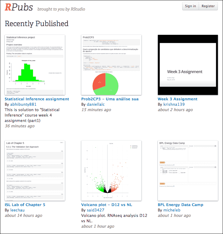
A screenshot of RPubs.com that contains some homework assginments submitted by students.
In a 2016 JSM (Joint Statistical Meetings) talk, I proposed that course instructors could sometimes intentionally insert some wrong values in the source data before providing it to the students for them to analyze the data in the homework, then correct these values the next time, and ask them to do the analysis again. This way, students should be able to realize the problems with the traditional cut-and-paste approach for data analysis (i.e., run the analysis separately and copy the results manually), and the advantage of using R Markdown to automatically generate the report.
Subsection 2.1.3 Personalized mail
One thing you should remember about R Markdown is that you can programmatically generate reports, although most of the time you may be just clicking the
Knit button in RStudio to generate a single report from a single source document. Being able to program reports is a super power of R Markdown.
Mine Çetinkaya-Rundel once wanted to create personalized handouts for her workshop participants. She used a template R Markdown file, and knitted it in a for-loop to generate 20 PDF files for the 20 participants. Each PDF contained both personalized information and common information. You may read the article
https://rmarkdown.rstudio.com/articles_mail_merge.html for the technical details.
Subsection 2.1.4 2017 Employer Health Benefits Survey
The 2017 Employer Health Benefits Survey was designed and analyzed by the Kaiser Family Foundation, NORC at the University of Chicago, and Health Research & Educational Trust. The full PDF report was written in R Markdown (with the bookdown package). It has a unique appearance, which was made possible by heavy customizations in the LaTeX template. This example shows you that if you really care about typesetting, you are free to apply your knowledge about LaTeX to create highly sophisticated reports from R Markdown.
Subsection 2.1.5 Journal articles
Chris Hartgerink explained how and why he used R Markdown to write dynamic research documents in the post at
https://elifesciences.org/labs/cad57bcf/composing-reproducible-manuscripts-using-r-markdown He published a paper titled "Too Good to be False: Nonsignificant Results Revisited" with two co-authors [2]. The manuscript was written in R Markdown, and results were dynamically generated from the code in R Markdown.
When checking the accuracy of P-values in the psychology literature, his colleagues and he found that P-values could be mistyped or miscalculated, which could lead to inaccurate or even wrong conclusions. If the P-values were dynamically generated and inserted instead of being manually copied from statistical programs, the chance for those problems to exist would be much lower.
Lowndes et al. [4] also shows that using R Markdown (and version control) not only enhances reproducibility, but also produces better scientific research in less time.
Subsection 2.1.6 Dashboards at eelloo
R Markdown is used at eelloo (
https://eelloo.nl) to design and generate research reports. Here is one of their examples (in Dutch): https://eelloo.nl/groepsrapportages-met-infographics/, where you can find gauges, bar charts, pie charts, wordclouds, and other types of graphs dynamically generated and embedded in dashboards.
Subsection 2.1.7 Books
We will introduce the R Markdown extension bookdown in Chapter 12. It is an R package that allows you to write books and long-form reports with multiple Rmd files. After this package was published, a large number of books have emerged. You can find a subset of them at
https://bookdown.org. Some of these books have been printed, and some only have free online versions.
There have also been students who wrote their dissertations/theses with bookdown, such as Ed Berry:
https://eddjberry.netlify.com/post/writing-your-thesis-with-bookdown. Chester Ismay has even provided an R package thesisdown that can render a thesis in various formats. Several other people have customized this package for their own institutions, such as Zhian N. Kamvar’s beaverdown and Ben Marwick’s huskydown.
Subsection 2.1.8 Websites
The blogdown package to be introduced in Chapter 10 can be used to build general-purpose websites (including blogs and personal websites) based on R Markdown. You may find tons of examples at
https://github.com/rbind or by searching on Twitter: https://twitter.com/search?q=blogdown Here are a few impressive websites that I can quickly think of off the top of my head:
-
Rob J Hyndman’s personal website:
https://robjhyndman.com(a very comprehensive academic website).
-
Amber Thomas’s personal website:
https://amber.rbind.io(a rich project portfolio).
-
Emi Tanaka’s personal website:
https://emitanaka.github.io(in particular, check out the beautiful showcase page).
-
"Live Free or Dichotomize" by Nick Strayer and Lucy D’Agostino McGowan:
http://livefreeordichotomize.com(the layout is elegant, and the posts are useful and practical).
Section 2.2 Compile an R Markdown document
The usual way to compile an R Markdown document is to click the Reproducibility is the main reason that RStudio uses a new R session to render your Rmd documents: in most cases, you may want your documents to continue to work the next time you open R, or in other people’s computing environments. See this StackOverflow answer if you want to know more.
Knit button as shown in Figure 2.1, and the corresponding keyboard shortcut is Ctrl + Shift + K (Cmd + Shift + K on macOS). Under the hood, RStudio calls the function rmarkdown::render() to render the document _in a new R session_. Please note the emphasis here, which often confuses R Markdown users. Rendering an Rmd document in a new R session means that _none of the objects in your current R session (e.g., those you created in your R console) are available to that session_.2
This is not strictly true, but mostly true. You may save objects in your current R session to a file, e.g.,
.RData, and load it in a new R session.
If you must render a document in the current R session, you can also call
rmarkdown::render() by yourself, and pass the path of the Rmd file to this function. The second argument of this function is the output format, which defaults to the first output format you specify in the YAML metadata (if it is missing, the default is html_document). When you have multiple output formats in the metadata, and do not want to use the first one, you can specify the one you want in the second argument, e.g., for an Rmd document foo.Rmd with the metadata:
output:
  html_document:
    toc: true
  pdf_document:
    keep_tex: true
You can render it to PDF via:
rmarkdown::render('foo.Rmd', 'pdf_document')
The function call gives you much more freedom (e.g., you can generate a series of reports in a loop), but you should bear reproducibility in mind when you render documents this way. Of course, you can start a new and clean R session by yourself, and call
rmarkdown::render() in that session. As long as you do not manually interact with that session (e.g., manually creating variables in the R console), your reports should be reproducible.
Another main way to work with Rmd documents is the R Markdown Notebooks, which will be introduced in Section 3.2. With notebooks, you can run code chunks individually and see results right inside the RStudio editor. This is a convenient way to interact or experiment with code in an Rmd document, because you do not have to compile the whole document. Without using the notebooks, you can still partially execute code chunks, but the execution only occurs in the R console, and the notebook interface presents results of code chunks right beneath the chunks in the editor, which can be a great advantage. Again, for the sake of reproducibility, you will need to compile the whole document eventually in a clean environment.
Lastly, I want to mention an "unofficial" way to compile Rmd documents: the function
xaringan::inf_mr(), or equivalently, the RStudio addin "Infinite Moon Reader". Obviously, this requires you to install the **xaringan** package [35], which is available on CRAN. The main advantage of this way is LiveReload: a technology that enables you to live preview the output as soon as you save the source document, and you do not need to hit the Knit button. The other advantage is that it compiles the Rmd document _in the current R session_, which may or may not be what you desire. Note that this method only works for Rmd documents that output to HTML, including HTML documents and presentations.
A few R Markdown extension packages, such as bookdown and **blogdown**, have their own way of compiling documents, and we will introduce them later.
Note that it is also possible to render a series of reports instead of single one from a single R Markdown source document. You can parameterize an R Markdown document, and generate different reports using different parameters. See Chapter 15 for details.
Section 2.3 Cheat sheets
RStudio has created a large number of cheat sheets, including the one-page R Markdown cheat sheet, which are freely available at
https://www.rstudio.com/resources/cheatsheets/ There is also a more detailed R Markdown reference guide. Both documents can be used as quick references after you become more familiar with R Markdown.
Section 2.4 Output formats
There are two types of output formats in the rmarkdown package: documents, and presentations. All available formats are listed below:
-
beamer_presentation -
context_document -
github_document -
html_document -
ioslides_presentation -
latex_document -
md_document -
odt_document -
pdf_document -
powerpoint_presentation -
rtf_document -
slidy_presentation -
word_document
We will document these output formats in detail in Chapter 3 and Chapter 4. There are more output formats provided in other extension packages (starting from Chapter 5). For the output format names in the YAML metadata of an Rmd file, you need to include the package name if a format is from an extension package, e.g.,
output: tufte::tufte_html
If the format is from the rmarkdown package, you do not need the
rmarkdown:: prefix (although it will not hurt).
When there are multiple output formats in a document, there will be a dropdown menu behind the RStudio
Knit button that lists the output format names (Figure 2.4).
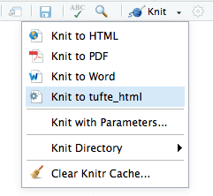
The output formats listed in the dropdown menu on the RStudio toolbar.
Each output format is often accompanied with several format options. All these options are documented on the R package help pages. For example, you can type
?rmarkdown::html_document in R to open the help page of the html_document format. When you want to use certain options, you have to translate the values from R to YAML, e.g.,
html_document(toc = TRUE, toc_depth = 2, dev = 'svg')
can be written in YAML as:
output:
  html_document:
    toc: true
    toc_depth: 2
    dev: 'svg'
The translation is often straightforward. Remember that R’s
TRUE, FALSE, and NULL are true, false, and null, respectively, in YAML. Character strings in YAML often do not require the quotes (e.g., dev: 'svg' and dev: svg are the same), unless they contain special characters, such as the colon :. If you are not sure if a string should be quoted or not, test it with the yaml package, e.g.,
cat(yaml::as.yaml(list(
  title = 'A Wonderful Day',
  subtitle = 'hygge: a quality of coziness'
)))
title: A Wonderful Day
subtitle: 'hygge: a quality of coziness'
Note that the subtitle in the above example is quoted because of the colon.
If you have options that need to be the result of an evaluated R expression, you can use
!expr, which tells the yaml package that it needs to parse and evaluate that option. Below is an example that uses a random theme for the HTML output:
output:
  html_document:
    theme: !expr sample(c("yeti", "united", "lumen"), 1)
If a certain option has sub-options (which means the value of this option is a list in R), the sub-options need to be further indented, e.g.,
output:
  html_document:
    toc: true
    includes:
      in_header: header.html
      before_body: before.html
Some options are passed to knitr, such as
dev, fig_width, and fig_height. Detailed documentation of these options can be found on the knitr documentation page: https://yihui.name/knitr/options/ Note that the actual knitr option names can be different. In particular, knitr uses . in names, but rmarkdown uses _, e.g., fig_width in rmarkdown corresponds to fig.width in knitr. We apologize for the inconsistencies---programmers often strive for consistencies in their own world, yet one standard plus one standard often equals three standards. If I were to design the knitr package again, I would definitely use _.
Some options are passed to Pandoc, such as
toc, toc_depth, and number_sections. You should consult the Pandoc documentation when in doubt. R Markdown output format functions often have a pandoc_args argument, which should be a character vector of extra arguments to be passed to Pandoc. If you find any Pandoc features that are not represented by the output format arguments, you may use this ultimate argument, e.g.,
output:
  pdf_document:
    toc: true
    pandoc_args: ["--wrap=none", "--top-level-division=chapter"]
Section 2.5 Markdown syntax
The text in an R Markdown document is written with the Markdown syntax. Precisely speaking, it is Pandoc’s Markdown. There are many flavors of Markdown invented by different people, and Pandoc’s flavor is the most comprehensive one to our knowledge. You can find the full documentation of Pandoc’s Markdown at
https://pandoc.org/MANUAL.html We strongly recommend that you read this page at least once to know all the possibilities with Pandoc’s Markdown, even if you will not use all of them. This section is adapted from Section 2.1 of [6], and only covers a small subset of Pandoc’s Markdown syntax.
Subsection 2.5.1 Inline formatting
Inline text will be italic if surrounded by underscores or asterisks, e.g.,
_text_ or *text*. Bold text is produced using a pair of double asterisks (**text**). A pair of tildes (~) turn text to a subscript (e.g., H~3~PO~4~ renders \(H_3PO_4\)). A pair of carets (^) produce a superscript (e.g., Cu^2+^ renders \(Cu^{2+}\)).
To mark text as
inline code, use a pair of backticks, e.g., `code`. To include \(n\) literal backticks, use at least \(n+1\) backticks outside, e.g., you can use four backticks to preserve three backtick inside: ```` ```code``` ````, which is rendered as ```code```.
Hyperlinks are created using the syntax
[text](link), e.g., [RStudio](https://www.rstudio.com). The syntax for images is similar: just add an exclamation mark, e.g., . Footnotes are put inside the square brackets after a caret ^[], e.g., ^[This is a footnote.].
There are multiple ways to insert citations, and we recommend that you use BibTeX databases, because they work better when the output format is LaTeX/PDF. Section 2.8 of [6] has explained the details. The key idea is that when you have a BibTeX database (a plain-text file with the conventional filename extension
.bib) that contains entries like:
@Manual{R-base,
  title = {R: A Language and Environment for Statistical
    Computing},
  author = {{R Core Team}},
  organization = {R Foundation for Statistical Computing},
  address = {Vienna, Austria},
  year = {2017},
  url = {https://www.R-project.org/},
}
You may add a field named
bibliography to the YAML metadata, and set its value to the path of the BibTeX file. Then in Markdown, you may use @R-base or [@R-base] to reference the BibTeX entry. Pandoc will automatically generate a list of references in the end of the document.
Subsection 2.5.2 Block-level elements
Section headers can be written after a number of pound signs, e.g.,
# First-level header

## Second-level header

### Third-level header
If you do not want a certain heading to be numbered, you can add
{-} or {.unnumbered} after the heading, e.g.,
# Preface {-}
Unordered list items start with
*, -, or +, and you can nest one list within another list by indenting the sub-list, e.g.,
- one item
- one item
- one item
    - one more item
    - one more item
    - one more item
The output is:
-
one item
-
one item
-
one item
-
one more item
-
one more item
-
one more item
-
Ordered list items start with numbers (you can also nest lists within lists), e.g.,
1. the first item
2. the second item
3. the third item
    - one unordered item
    - one unordered item
The output does not look too much different with the Markdown source:
-
the first item
-
the second item
-
the third item
-
one unordered item
-
one unordered item
-
Blockquotes are written after
>, e.g.,
> "I thoroughly disapprove of duels. If a man should challenge me,
  I would take him kindly and forgivingly by the hand and lead him
  to a quiet place and kill him."
>
> --- Mark Twain
The actual output (we customized the style for blockquotes in this book):
> "I thoroughly disapprove of duels. If a man should challenge me, I would take him kindly and forgivingly by the hand and lead him to a quiet place and kill him." > > --- Mark Twain
Plain code blocks can be written after three or more backticks, and you can also indent the blocks by four spaces, e.g.,
```
This text is displayed verbatim / preformatted
```

Or indent by four spaces:

    This text is displayed verbatim / preformatted
In general, you’d better leave at least one empty line between adjacent but different elements, e.g., a header and a paragraph. This is to avoid ambiguity to the Markdown renderer. For example, does "
#" indicate a header below?
In R, the character
# indicates a comment.
And does "
-" mean a bullet point below?
The result of 5
- 3 is 2.
Different flavors of Markdown may produce different results if there are no blank lines.
Subsection 2.5.3 Math expressions
Inline LaTeX equations can be written in a pair of dollar signs using the LaTeX syntax, e.g.,
$f(k) = {n \choose k} p^{k} (1-p)^{n-k}$ (actual output: \(f(k)={n \choose k}p^{k}(1-p)^{n-k}\)); math expressions of the display style can be written in a pair of double dollar signs, e.g., $$f(k) = {n \choose k} p^{k} (1-p)^{n-k}$$, and the output looks like this:
\begin{equation*}
f\left(k\right)=\binom{n}{k}p^k\left(1-p\right)^{n-k}
\end{equation*}
$$\begin{array}{ccc}
x_{11} & x_{12} & x_{13}\\
x_{21} & x_{22} & x_{23}
\end{array}$$
\begin{equation*}
\begin{array}{ccc} x_{11} & x_{12} & x_{13}\\ x_{21} & x_{22} & x_{23} \end{array}
\end{equation*}
$$X = \begin{bmatrix}1 & x_{1}\\
1 & x_{2}\\
1 & x_{3}
\end{bmatrix}$$
\begin{equation*}
X = \begin{bmatrix}1 & x_{1}\\ 1 & x_{2}\\ 1 & x_{3} \end{bmatrix}
\end{equation*}
$$\Theta = \begin{pmatrix}\alpha & \beta\\
\gamma & \delta
\end{pmatrix}$$
\begin{equation*}
\Theta = \begin{pmatrix}\alpha & \beta\\ \gamma & \delta \end{pmatrix}
\end{equation*}
$$\begin{vmatrix}a & b\\
c & d
\end{vmatrix}=ad-bc$$
\begin{equation*}
\begin{vmatrix}a & b\\ c & d \end{vmatrix}=ad-bc
\end{equation*}
Section 2.6 R code chunks and inline R code
You can insert an R code chunk either using the RStudio toolbar (the
Insert button) or the keyboard shortcut Ctrl + Alt + I (Cmd + Option + I on macOS).
There are a lot of things you can do in a code chunk: you can produce text output, tables, or graphics. You have fine control over all these output via chunk options, which can be provided inside the curly braces (between
```{r and }). For example, you can choose hide text output via the chunk option results = 'hide', or set the figure height to 4 inches via fig.height = 4`. Chunk options are separated by commas, e.g.,
```{r, chunk-label, results='hide', fig.height=4}
The value of a chunk option can be an arbitrary R expression, which makes chunk options extremely flexible. For example, the chunk option
eval controls whether to evaluate (execute) a code chunk, and you may conditionally evaluate a chunk via a variable defined previously, e.g.,
```{r}
# execute code if the date is later than a specified day
do_it = Sys.Date() > '2018-02-14'
```

```{r, eval=do_it}
x = rnorm(100)
```
There are a large number of chunk options in knitr documented at https://yihui.name/knitr/options We list a subset of them below:
-
eval: Whether to evaluate a code chunk.
-
echo: Whether to echo the source code in the output document (someone may not prefer reading your smart source code but only results).
-
results: When set to'hide', text output will be hidden; when set to'asis', text output is written "as-is", e.g., you can write out raw Markdown text from R code (likecat('**Markdown** is cool.\n')). By default, text output will be wrapped in verbatim elements (typically plain code blocks).
-
collapse: Whether to merge text output and source code into a single code block in the output. This is mostly cosmetic:collapse = TRUEmakes the output more compact, since the R source code and its text output are displayed in a single output block. The defaultcollapse = FALSEmeans R expressions and their text output are separated into different blocks.
-
warning,message, anderror: Whether to show warnings, messages, and errors in the output document. Note that if you seterror = FALSE,rmarkdown::render()will halt on error in a code chunk, and the error will be displayed in the R console. Similarly, whenwarning = FALSEormessage = FALSE, these messages will be shown in the R console.
-
include: Whether to include anything from a code chunk in the output document. Wheninclude = FALSE, this whole code chunk is excluded in the output, but note that it will still be evaluated ifeval = TRUE. When you are trying to setecho = FALSE,results = 'hide',warning = FALSE, andmessage = FALSE, chances are you simply mean a single optioninclude = FALSEinstead of suppressing different types of text output individually.
-
cache: Whether to enable caching. If caching is enabled, the same code chunk will not be evaluated the next time the document is compiled (if the code chunk was not modified), which can save you time. However, I want to honestly remind you of the two hard problems in computer science (via Phil Karlton): naming things, and cache invalidation. Caching can be handy but also tricky sometimes.
-
fig.widthandfig.height: The (graphical device) size of R plots in inches. R plots in code chunks are first recorded via a graphical device in knitr, and then written out to files. You can also specify the two options together in a single chunk optionfig.dim, e.g.,fig.dim = c(6, 4)meansfig.width = 6andfig.height = 4.
-
out.widthandout.height: The output size of R plots in the output document. These options may scale images. You can use percentages, e.g.,out.width = '80%'means 80% of the page width.
-
dev: The graphical device to record R plots. Typically it is'pdf'for LaTeX output, and'png'for HTML output, but you can certainly use other devices, such as'svg'or'jpeg'.
-
fig.cap: The figure caption.
-
child: You can include a child document in the main document. This option takes a path to an external file.
Chunk options in knitr can be surprisingly powerful. For example, you can create animations from a series of plots in a code chunk. I will not explain how here because it requires an external software package, but encourage you to read the documentation carefully to discover the possibilities. You may also read [5], which is a comprehensive guide to the knitr package, but unfortunately biased towards LaTeX users for historical reasons (which was one of the reasons why I wanted to write this R Markdown book).
There is an optional chunk option that does not take any value, which is the chunk label. It should be the first option in the chunk header. Chunk labels are mainly used in filenames of plots and cache. If the label of a chunk is missing, a default one of the form
unnamed-chunk-i will be generated, where i is incremental. I strongly recommend that you only use alphanumeric characters (a-z, A-Z and 0-9) and dashes (-) in labels, because they are not special characters and will surely work for all output formats. Other characters, spaces and underscores in particular, may cause trouble in certain packages, such as bookdown.
If a certain option needs to be frequently set to a value in multiple code chunks, you can consider setting it globally in the first code chunk of your document, e.g.,
```{r, setup, include=FALSE}
knitr::opts_chunk$set(fig.width = 8, collapse = TRUE)
```
Besides code chunks, you can also insert values of R objects inline in text. For example:
```{r}
x = 5  # radius of a circle
```

For a circle with the radius `r  x'`,
its area is `r pi * x^2`
Subsection 2.6.1 Figures
By default, figures produced by R code will be placed immediately after the code chunk they were generated from. For example:
```{r}
plot(cars, pch = 18)
```
You can provide a figure caption using
fig.cap in the chunk options. If the document output format supports the option fig_caption: true (e.g., the output format rmarkdown::html_document), the R plots will be placed into figure environments. In the case of PDF output, such figures will be automatically numbered. If you also want to number figures in other formats (such as HTML), please see the bookdown package in Chapter 12 (in particular, see Subsection 12.4.4).
PDF documents are generated through the LaTeX files generated from R Markdown. A highly surprising fact to LaTeX beginners is that figures float by default: even if you generate a plot in a code chunk on the first page, the whole figure environment may float to the next page. This is just how LaTeX works by default. It has a tendency to float figures to the top or bottom of pages. Although it can be annoying and distracting, we recommend that you refrain from playing the "Whac-A-Mole" game in the beginning of your writing, i.e., desparately trying to position figures "correctly" while they seem to be always dodging you. You may wish to fine-tune the positions once the content is complete using the
fig.pos chunk option (e.g., fig.pos = 'h'). See https://www.overleaf.com/learn/latex/Positioning_images_and_tables for possible values of fig.pos and more general tips about this behavior in LaTeX. In short, this can be a difficult problem for PDF output.
To place multiple figures side-by-side from the same code chunk, you can use the
fig.show='hold' option along with the out.width option. Figure 2.5 shows an example with two plots, each with a width of 50%.
par(mar = c(4, 4, .2, .1))
plot(cars, pch = 19)
plot(pressure, pch = 17)
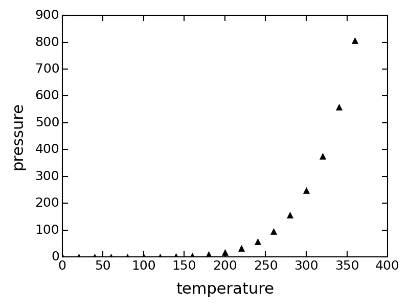
Two plots side-by-side, each with a width of 50%.
If you want to include a graphic that is not generated from R code, you may use the
knitr::include_graphics() function, which gives you more control over the attributes of the image than the Markdown syntax of  (e.g., you can specify the image width via out.width). Figure 2.6 provides an example of this.
```{r, out.width='25%', fig.align='center', fig.cap='...'}
knitr::include_graphics('images/hex-rmarkdown.png')
```

The R Markdown hex logo.
Subsection 2.6.2 Tables
The easiest way to include tables is by using Table captions can be included by passing
knitr::kable(), which can create tables for HTML, PDF and Word outputs.3
You may also consider the pander package. There are several other packages for producing tables, including xtable, Hmisc, and stargazer, but these are generally less compatible with multiple output formats.
caption to the function, e.g.,
```{r tables-mtcars}
knitr::kable(iris[1:5, ], caption = 'A caption')
```
Tables in non-LaTeX output formats will always be placed after the code block. For LaTeX/PDF output formats, tables have the same issue as figures: they may float. If you want to avoid this behavior, you will need to use the LaTeX package longtable, which can break tables across multiple pages. This can be achieved by adding
\usepackage{longtable} to your LaTeX preamble, and passing longtable = TRUE to kable().
If you are looking for more advanced control of the styling of tables, you are recommended to use the kableExtra package, which provides functions to customize the appearance of PDF and HTML tables. Formatting tables can be a very complicated task, especially when certain cells span more than one column or row. It is even more complicated when you have to consider different output formats. For example, it is difficult to make a complex table work for both PDF and HTML output. We know it is disappointing, but sometimes you may have to consider alternative ways of presenting data, such as using graphics.
We explain in Section 12.3 how the bookdown package extends the functionality of rmarkdown to allow for figures and tables to be easily cross-referenced within your text.
Section 2.7 Other language engines
A less well-known fact about R Markdown is that many other languages are also supported, such as Python, Julia, C++, and SQL. The support comes from the knitr package, which has provided a large number of _language engines_. Language engines are essentially functions registered in the object
knitr::knit_engine. You can list the names of all available engines via:
names(knitr::knit_engines$get())
##  [1] "awk"          "bash"         "coffee"
##  [4] "gawk"         "groovy"       "haskell"
##  [7] "lein"         "mysql"        "node"
## [10] "octave"       "perl"         "php"
## [13] "psql"         "Rscript"      "ruby"
## [16] "sas"          "scala"        "sed"
## [19] "sh"           "stata"        "zsh"
## [22] "asis"         "asy"          "block"
## [25] "block2"       "bslib"        "c"
## [28] "cat"          "cc"           "comment"
## [31] "css"          "ditaa"        "dot"
## [34] "embed"        "eviews"       "exec"
## [37] "fortran"      "fortran95"    "go"
## [40] "highlight"    "js"           "julia"
## [43] "python"       "R"            "Rcpp"
## [46] "sass"         "scss"         "sql"
## [49] "stan"         "targets"      "tikz"
## [52] "verbatim"     "theorem"      "lemma"
## [55] "corollary"    "proposition"  "conjecture"
## [58] "definition"   "example"      "exercise"
## [61] "hypothesis"   "proof"        "remark"
## [64] "solution"     "marginfigure"
Most engines have been documented in Chapter 11 of [5]. The engines from
theorem to solution are only available when you use the bookdown package, and the rest are shipped with the knitr package. To use a different language engine, you can change the language name in the chunk header from r to the engine name, e.g.,
```{python}
x = 'hello, python world!'
print(x.split(' '))
```
For engines that rely on external interpreters such as
python, perl, and ruby, the default interpreters are obtained from Sys.which(), i.e., using the interpreter found via the environment variable PATH of the system. If you want to use an alternative interpreter, you may specify its path in the chunk option engine.path. For example, you may want to use Python 3 instead of the default Python 2, and we assume Python 3 is at /usr/bin/python3 (may not be true for your system):
```{python, engine.path = '/usr/bin/python3'}
import sys
print(sys.version)
```
You can also change the engine interpreters globally for multiple engines, e.g.,
knitr::opts_chunk$set(engine.path = list(
  python = '~/anaconda/bin/python',
  ruby = '/usr/local/bin/ruby'
))
Note that you can use a named list to specify the paths for different engines.
Most engines will execute each code chunk in a separate new session (via a
system() call in R), which means objects created in memory in a previous code chunk will not be directly available to latter code chunks. For example, if you create a variable in a bash code chunk, you will not be able to use it in the next bash code chunk. Currently the only exceptions are r, python, and julia. Only these engines execute code in the same session throughout the document. To clarify, all r code chunks are executed in the same R session, all python code chunks are executed in the same Python session, and so on, but the R session and the Python session are independent.4
This is not strictly true, since the Python session is actually launched from R. What I mean here is that you should not expect to use R variables and Python variables interchangeably without explicitly importing/exporting variables between the two sessions.
I will introduce some specific features and examples for a subset of language engines in knitr below. Note that most chunk options should work for both R and other languages, such as
eval and echo, so these options will not be mentioned again.
Subsection 2.7.1 Python
The
python engine is based on the reticulate package [24], which makes it possible to execute all Python code chunks in the same Python session. If you actually want to execute a certain code chunk in a new Python session, you may use the chunk option python.reticulate = FALSE. If you are using a knitr version lower than 1.18, you should update your R packages.
Below is a relatively simple example that shows how you can create/modify variables, and draw graphics in Python code chunks. Values can be passed to or retrieved from the Python session. To pass a value to Python, assign to
py$name, where name is the variable name you want to use in the Python session; to retrieve a value from Python, also use py$name.
---
title: "Python code chunks in R Markdown"
date: 2018-02-22
---

## A normal R code chunk

```{r}
library(reticulate)
x = 42
print(x)
```

## Modify an R variable

In the following chunk, the value of `x` on the right hand side
is `r x`, which was defined in the previous chunk.

```{r}
x = x + 12
print(x)
```

## A Python chunk

This works fine and as expected.

```{python}
x = 42 * 2
print(x)
```

The value of `x` in the Python session is `r py$x`.
It is not the same `x` as the one in R.

## Modify a Python variable

```{python}
x = x + 18
print(x)
```

Retrieve the value of `x` from the Python session again:

```{r}
py$x
```

Assign to a variable in the Python session from R:

```{r}
py$y = 1:5
```

See the value of `y` in the Python session:

```{python}
print(y)
```

## Python graphics

You can draw plots using the **matplotlib** package in Python.

```{python}
import matplotlib.pyplot as plt
plt.plot([0, 2, 1, 4])
plt.show()
```
You may learn more about the reticulate package from https://rstudio.github.io/reticulate/
Subsection 2.7.2 Shell scripts
You can also write Shell scripts in R Markdown, if your system can run them (the executable
bash or sh should exist). Usually this is not a problem for Linux or macOS users. It is not impossible for Windows users to run Shell scripts, but you will have to install additional software (such as Cygwin or the Linux Subsystem).
```{bash}
echo "Hello Bash!"
cat flights1.csv flights2.csv flights3.csv > flights.csv
```
Shell scripts are executed via the
system2() function in R. Basically knitr passes a code chunk to the command bash -c to run it.
Subsection 2.7.3 SQL
The
sql engine uses the DBI package to execute SQL queries, print their results, and optionally assign the results to a data frame.
To use the
sql engine, you first need to establish a DBI connection to a database (typically via the DBI::dbConnect() function). You can make use of this connection in a sql chunk via the connection option. For example:
```{r}
library(DBI)
db = dbConnect(RSQLite::SQLite(), dbname = "sql.sqlite")
```

```{sql, connection=db}
SELECT * FROM trials
```
By default,
SELECT queries will display the first 10 records of their results within the document. The number of records displayed is controlled by the max.print option, which is in turn derived from the global knitr option sql.max.print (e.g., knitr::opts_knit$set(sql.max.print = 10); N.B. it is opts_knit instead of opts_chunk). For example, the following code chunk displays the first 20 records:
```{sql, connection=db, max.print = 20}
SELECT * FROM trials
```
By default, the
sql engine includes a caption that indicates the total number of records displayed. You can override this caption using the tab.cap chunk option. For example:
```{sql, connection=db, tab.cap = "My Caption"}
SELECT * FROM trials
```
You can specify that you want no caption all via
tab.cap = NA.
If you want to assign the results of the SQL query to an R object as a data frame, you can do this using the
output.var option, e.g.,
```{sql, connection=db, output.var="trials"}
SELECT * FROM trials
```
When the results of a SQL query are assigned to a data frame, no records will be printed within the document (if desired, you can manually print the data frame in a subsequent R chunk).
If you need to bind the values of R variables into SQL queries, you can do so by prefacing R variable references with a
?. For example:
```{r}
subjects = 10
```

```{sql, connection=db, output.var="trials"}
SELECT * FROM trials WHERE subjects >= ?subjects
```
If you have many SQL chunks, it may be helpful to set a default for the
connection chunk option in the setup chunk, so that it is not necessary to specify the connection on each individual chunk. You can do this as follows:
```{r setup}
library(DBI)
db = dbConnect(RSQLite::SQLite(), dbname = "sql.sqlite")
knitr::opts_chunk$set(connection = "db")
```
Note that the
connection option should be a string naming the connection object (not the object itself). Once set, you can execute SQL chunks without specifying an explicit connection:
```{sql}
SELECT * FROM trials
```
Subsection 2.7.4 Rcpp
The
Rcpp engine enables compilation of C++ into R functions via the Rcpp sourceCpp() function. For example:
```{rcpp}
#include <Rcpp.h>
using namespace Rcpp;

// [[Rcpp::export]]
NumericVector timesTwo(NumericVector x) {
  return x * 2;
}
```
Executing this chunk will compile the code and make the C++ function
timesTwo() available to R.
You can cache the compilation of C++ code chunks using standard knitr caching, i.e., add the
cache = TRUE option to the chunk:
```{Rcpp, cache=TRUE}
#include <Rcpp.h>
using namespace Rcpp;

// [[Rcpp::export]]
NumericVector timesTwo(NumericVector x) {
  return x * 2;
}
```
In some cases, it is desirable to combine all of the
Rcpp code chunks in a document into a single compilation unit. This is especially useful when you want to intersperse narrative between pieces of C++ code (e.g., for a tutorial or user guide). It also reduces total compilation time for the document (since there is only a single invocation of the C++ compiler rather than multiple).
To combine all Rcpp chunks into a single compilation unit, you use the
ref.label chunk option along with the knitr::all_rcpp_labels() function to collect all of the Rcpp chunks in the document. Here is a simple example:
All C++ code chunks will be combined to the chunk below:

```{rcpp, ref.label=knitr::all_rcpp_labels(), include=FALSE}
```

First we include the header `Rcpp.h`:

```{rcpp, eval=FALSE}
#include <Rcpp.h>
```

Then we define a function:

```{rcpp, eval=FALSE}
// [[Rcpp::export]]
int timesTwo(int x) {
  return x * 2;
}
```
The two
Rcpp chunks that include code will be collected and compiled together in the first Rcpp chunk via the ref.label chunk option. Note that we set the eval = FALSE option on the Rcpp chunks with code in them to prevent them from being compiled again.
Subsection 2.7.5 Stan
The
stan engine enables embedding of the Stan probabilistic programming language within R Markdown documents.
The Stan model within the code chunk is compiled into a
stanmodel object, and is assigned to a variable with the name given by the output.var option. For example:
```{stan, output.var="ex1"}
parameters {
  real y[2];
}
model {
  y[1] ~ normal(0, 1);
  y[2] ~ double_exponential(0, 2);
}
```

```{r}
library(rstan)
fit = sampling(ex1)
print(fit)
```
Subsection 2.7.6 JavaScript and CSS
If you are using an R Markdown format that targets HTML output (e.g.,
html_document and ioslides_presentation, etc.), you can include JavaScript to be executed within the HTML page using the JavaScript engine named js.
For example, the following chunk uses jQuery (which is included in most R Markdown HTML formats) to change the color of the document title to red:
```{js, echo=FALSE}
$('.title').css('color', 'red')
```
Similarly, you can embed CSS rules in the output document. For example, the following code chunk turns text within the document body red:
```{css, echo=FALSE}
body {
  color: red;
}
```
Without the chunk option
echo = FALSE, the JavaScript/CSS code will be displayed verbatim in the output document, which is probably not what you want.
Subsection 2.7.7 Julia
The Julia language is supported through the JuliaCall package [18]. Similar to the
python engine, the julia engine runs all Julia code chunks in the same Julia session. Below is a minimal example:
```{julia}
a = sqrt(2);  # the semicolon inhibits printing
```
Subsection 2.7.8 C and Fortran
For code chunks that use C or Fortran, knitr uses
R CMD SHLIB to compile the code, and load the shared object (a *.so file on Unix or *.dll on Windows). Then you can use .C() / .Fortran() to call the C / Fortran functions, e.g.,
```{c, test-c, results='hide'}
void square(double *x) {
  *x = *x * *x;
}
```

Test the `square()` function:

```{r}
.C('square', 9)
.C('square', 123)
```
You can find more examples on different language engines in the GitHub repository https://github.com/yihui/knitr-examples (look for filenames that contain the word "engine").
Section 2.8 Interactive documents
R Markdown documents can also generate interactive content. There are two types of interactive R Markdown documents: you can use the HTML Widgets framework, or the Shiny framework (or both). They will be described in more detail in Chapter 16 and Chapter 19, respectively.
Subsection 2.8.1 HTML widgets
The HTML Widgets framework is implemented in the R package htmlwidgets [17], interfacing JavaScript libraries that create interactive applications, such as interactive graphics and tables. Several widget packages have been developed based on this framework, such as DT [13], leaflet [19], and dygraphs [14]. Visit
https://www.htmlwidgets.org to know more about widget packages as well as how to develop a widget package by yourself.
Figure 2.7 shows an interactive map created via the leaflet package, and the source document is below:
---
title: "An Interactive Map"
---

Below is a map that shows the location of the
Department of Statistics, Iowa State University.

```{r out.width='100%', echo=FALSE}
library(leaflet)
leaflet() %>% addTiles() %>%
  setView(-93.65, 42.0285, zoom = 17) %>%
  addPopups(
    -93.65, 42.0285,
    'Here is the <b>Department of Statistics</b>, ISU'
  )
```
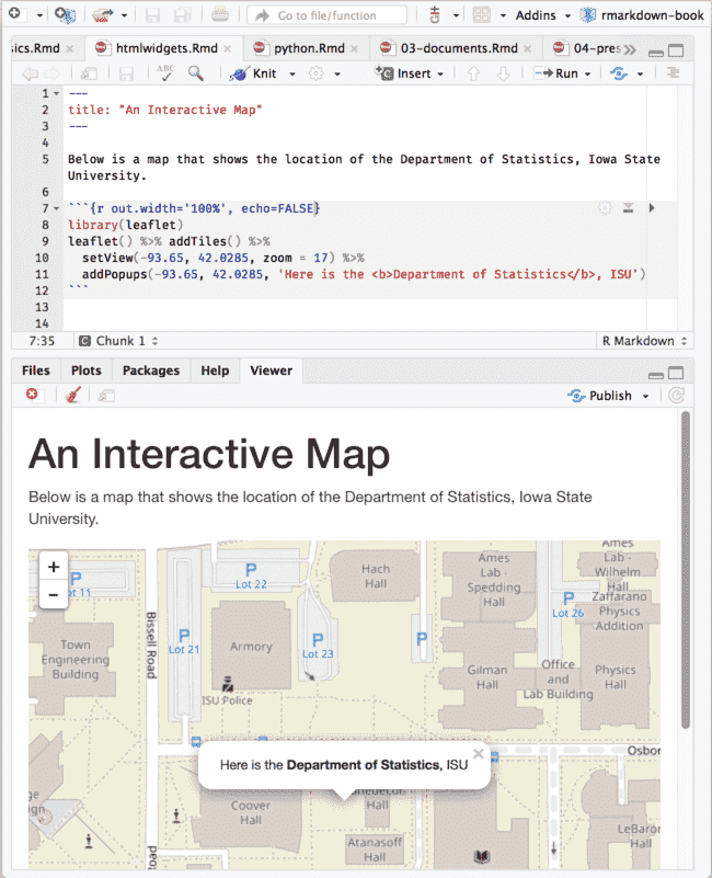
An R Markdown document with a leaflet map widget.
Although HTML widgets are based on JavaScript, the syntax to create them in R is often pure R syntax.
If you include an HTML widget in a non-HTML output format, such as a PDF, knitr will try to embed a screenshot of the widget if you have installed the R package webshot [34] and the PhantomJS package (via
webshot::install_phantomjs()).
Subsection 2.8.2 Shiny documents
The shiny package [29] builds interactive web apps powered by R. To call Shiny code from an R Markdown document, add
runtime: shiny to the YAML metadata, like in this document:
---
title: "A Shiny Document"
output: html_document
runtime: shiny
---

A standard R plot can be made interactive by wrapping
it in the Shiny `renderPlot()` function. The `selectInput()`
function creates the input widget to drive the plot.

```{r eruptions, echo=FALSE}
selectInput(
  'breaks', label = 'Number of bins:',
  choices = c(10, 20, 35, 50), selected = 20
)

renderPlot({
  par(mar = c(4, 4, .1, .5))
  hist(
    faithful$eruptions, as.numeric(input$breaks),
    col = 'gray', border = 'white',
    xlab = 'Duration (minutes)', main = ''
  )
})
```
Figure 2.8 shows the output, where you can see a dropdown menu that allows you to choose the number of bins in the histogram.
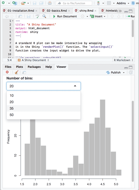
An R Markdown document with a Shiny widget.
You may use Shiny to run any R code that you like in response to user actions. Since web browsers cannot execute R code, Shiny interactions occur on the server side and rely on a live R session. By comparison, HTML widgets do not require a live R session to support them, because the interactivity comes from the client side (via JavaScript in the web browser).
You can learn more about Shiny at
https://shiny.rstudio.com
HTML widgets and Shiny elements rely on HTML and JavaScript. They will work in any R Markdown format that is viewed in a web browser, such as HTML documents, dashboards, and HTML5 presentations.
