Chapter 3 Documents
The very original version of Markdown was invented mainly to write HTML content more easily. For example, you can write a bullet with
- text instead of the verbose HTML code <ul><li>text</li></ul>, or a quote with > text instead of <blockquote>text</blockquote>.
The syntax of Markdown has been greatly extended by Pandoc. What is more, Pandoc makes it possible to convert a Markdown document to a large variety of output formats. In this chapter, we will introduce the features of various document output formats. In the next two chapters, we will document the presentation formats and other R Markdown extensions, respectively.
Section 3.1 HTML document
As we just mentioned before, Markdown was originally designed for HTML output, so it may not be surprising that the HTML format has the richest features among all output formats. We recommend that you read this full section before you learn other output formats, because other formats have several features in common with the HTML document format, and we will not repeat these features in the corresponding sections.
To create an HTML document from R Markdown, you specify the
html_document output format in the YAML metadata of your document:
---
title: Habits
author: John Doe
date: March 22, 2005
output: html_document
---
Subsection 3.1.1 Table of contents
You can add a table of contents (TOC) using the
toc option and specify the depth of headers that it applies to using the toc_depth option. For example:
---
title: "Habits"
output:
  html_document:
    toc: true
    toc_depth: 2
---
If the table of contents depth is not explicitly specified, it defaults to 3 (meaning that all level 1, 2, and 3 headers will be included in the table of contents).
Subsubsection 3.1.1.1 Floating TOC
You can specify the
toc_float option to float the table of contents to the left of the main document content. The floating table of contents will always be visible even when the document is scrolled. For example:
---
title: "Habits"
output:
  html_document:
    toc: true
    toc_float: true
---
You may optionally specify a list of options for the
toc_float parameter which control its behavior. These options include:
-
collapsed(defaults toTRUE) controls whether the TOC appears with only the top-level (e.g., H2) headers. If collapsed initially, the TOC is automatically expanded inline when necessary. -
smooth_scroll(defaults toTRUE) controls whether page scrolls are animated when TOC items are navigated to via mouse clicks. For example:
---
title: "Habits"
output:
  html_document:
    toc: true
    toc_float:
      collapsed: false
      smooth_scroll: false
---
Subsection 3.1.2 Section numbering
You can add section numbering to headers using the
number_sections option:
---
title: "Habits"
output:
  html_document:
    toc: true
    number_sections: true
---
Note that if you do choose to use the
number_sections option, you will likely also want to use # (H1) headers in your document as ## (H2) headers will include a decimal point, because without H1 headers, you H2 headers will be numbered with 0.1, 0.2, and so on.
Subsection 3.1.3 Tabbed sections
You can organize content using tabs by applying the
.tabset class attribute to headers within a document. This will cause all sub-headers of the header with the .tabset attribute to appear within tabs rather than as standalone sections. For example:
## Quarterly Results {.tabset}

### By Product

(tab content)

### By Region

(tab content)
You can also specify two additional attributes to control the appearance and behavior of the tabs. The
.tabset-fade attribute causes the tabs to fade in and out when switching between tabs. The .tabset-pills attribute causes the visual appearance of the tabs to be "pill" (see Figure 3.1) rather than traditional tabs. For example:
## Quarterly Results {.tabset .tabset-fade .tabset-pills}
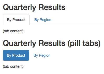
Traditional tabs and pill tabs on an HTML page.
Subsection 3.1.4 Appearance and style
There are several options that control the appearance of HTML documents:
-
themespecifies the Bootstrap theme to use for the page (themes are drawn from the Bootswatch theme library). Valid themes includer knitr::combine_words(rmarkdown:::themes()). Passnullfor no theme (in this case you can use thecssparameter to add your own styles). -
highlightspecifies the syntax highlighting style. Supported styles includer knitr::combine_words(rmarkdown:::html_highlighters(), before='\x60'). Passnullto prevent syntax highlighting. -
smartindicates whether to produce typographically correct output, converting straight quotes to curly quotes,---to em-dashes,--to en-dashes, and...to ellipses. Note thatsmartis enabled by default. For example:
---
title: "Habits"
output:
  html_document:
    theme: united
    highlight: tango
---
Subsubsection 3.1.4.1 Custom CSS
You can add your own CSS to an HTML document using the
css option:
---
title: "Habits"
output:
  html_document:
    css: styles.css
---
If you want to provide all of the styles for the document from your own CSS you set the
theme (and potentially highlight) to null:
---
title: "Habits"
output:
  html_document:
    theme: null
    highlight: null
    css: styles.css
---
You can also target specific sections of documents with custom CSS by adding ids or classes to section headers within your document. For example the following section header:
## Next Steps {#nextsteps .emphasized}
Would enable you to apply CSS to all of its content using either of the following CSS selectors:
#nextsteps {
   color: blue;
}

.emphasized {
   font-size: 1.2em;
}
Subsection 3.1.5 Figure options
There are a number of options that affect the output of figures within HTML documents:
-
fig_widthandfig_heightcan be used to control the default figure width and height (7x5 is used by default). -
fig_retinaspecifies the scaling to perform for retina displays (defaults to 2, which currently works for all widely used retina displays). Set tonullto prevent retina scaling. -
fig_captioncontrols whether figures are rendered with captions.
---
title: "Habits"
output:
  html_document:
    fig_width: 7
    fig_height: 6
    fig_caption: true
---
Subsection 3.1.6 Data frame printing
You can enhance the default display of data frames via the
df_print option. Valid values are shown in Table 3.2.
| Option | Description |
|---|---|
default |
Call the print.data.frame generic method |
kable |
Use the knitr::kable function |
tibble |
Use the tibble::print.tbl_df function |
paged |
Use rmarkdown::paged_table to create a pageable table |
| A custom function | Use the function to create the table |
Subsubsection 3.1.6.1 Paged printing
When the
df_print option is set to paged, tables are printed as HTML tables with support for pagination over rows and columns. For instance (see Figure 3.3):
---
title: "Motor Trend Car Road Tests"
output:
  html_document:
    df_print: paged
---

```{r}
mtcars
```
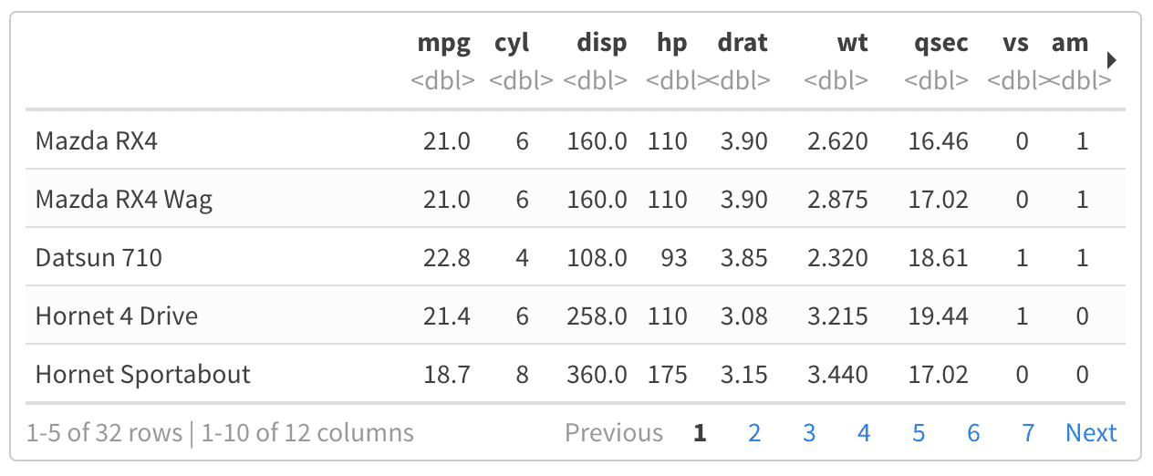
A paged table in the HTML output document.
| Option | Description |
|---|---|
max.print |
The number of rows to print. |
rows.print |
The number of rows to display. |
cols.print |
The number of columns to display. |
cols.min.print |
The minimum number of columns to display. |
pages.print |
The number of pages to display under page navigation. |
paged.print |
When set to FALSE turns off paged tables. |
rownames.print |
When set to FALSE turns off row names. |
These options are specified in each chunk like below:
```{r cols.print=3, rows.print=3}
mtcars
```
Subsubsection 3.1.6.2 Custom function
The
df_print option can also take an arbitrary function to create the table in the output document. This function must output in the correct format according to the output used.
For example,
rmarkdown::html_document(df_print = knitr::kable)
is the equivalent to using the method
"kable"
rmarkdown::html_document(df_print = "kable")
To use a custom function in
df_print within the YAML header, the tag !expr must be used so the R expression after it will be evaluated. See the eval.expr argument on the help page ?yaml::yaml.load for details.
---
title: "Motor Trend Car Road Tests"
output:
  html_document:
    df_print: !expr pander::pander
---

```{r}
mtcars
```
Subsection 3.1.7 Code folding
When the knitr chunk option
echo = TRUE is specified (the default behavior), the R source code within chunks is included within the rendered document. In some cases, it may be appropriate to exclude code entirely (echo = FALSE) but in other cases you might want the code to be available but not visible by default.
The
code_folding: hide option enables you to include R code but have it hidden by default. Users can then choose to show hidden R code chunks either individually or document wide. For example:
---
title: "Habits"
output:
  html_document:
    code_folding: hide
---
You can specify
code_folding: show to still show all R code by default but then allow users to hide the code if they wish.
Subsection 3.1.8 MathJax equations
By default, )MathJax scripts are included in HTML documents for rendering LaTeX and MathML equations. You can use the
mathjax option to control how MathJax is included:
-
Specify
"default"to use an HTTPS URL from a CDN host (currently provided by RStudio). -
Specify
"local"to use a local version of MathJax (which is copied into the output directory). Note that when using"local"you also need to set theself_containedoption tofalse. -
Specify an alternate URL to load MathJax from another location.
-
Specify
nullto exclude MathJax entirely. For example, to use a local copy of MathJax:
---
title: "Habits"
output:
  html_document:
    mathjax: local
    self_contained: false
---
To use a self-hosted copy of MathJax:
---
title: "Habits"
output:
  html_document:
    mathjax: "http://example.com/MathJax.js"
---
To exclude MathJax entirely:
---
title: "Habits"
output:
  html_document:
    mathjax: null
---
Subsection 3.1.9 Document dependencies
By default, R Markdown produces standalone HTML files with no external dependencies, using
data: URIs to incorporate the contents of linked scripts, stylesheets, images, and videos. This means you can share or publish the file just like you share Office documents or PDFs. If you would rather keep dependencies in external files, you can specify self_contained: false. For example:
---
title: "Habits"
output:
  html_document:
    self_contained: false
---
Note that even for self-contained documents, MathJax is still loaded externally (this is necessary because of its big size). If you want to serve MathJax locally, you should specify
mathjax: local and self_contained: false.
One common reason to keep dependencies external is for serving R Markdown documents from a website (external dependencies can be cached separately by browsers, leading to faster page load times). In the case of serving multiple R Markdown documents you may also want to consolidate dependent library files (e.g. Bootstrap, and MathJax, etc.) into a single directory shared by multiple documents. You can use the
lib_dir option to do this. For example:
---
title: "Habits"
output:
  html_document:
    self_contained: false
    lib_dir: libs
---
Subsection 3.1.10 Advanced customization
Subsubsection 3.1.10.1 Keeping Markdown
When knitr processes an R Markdown input file, it creates a Markdown (
*.md) file that is subsequently transformed into HTML by Pandoc. If you want to keep a copy of the Markdown file after rendering, you can do so using the keep_md option:
---
title: "Habits"
output:
  html_document:
    keep_md: true
---
Subsubsection 3.1.10.2 Includes
You can do more advanced customization of output by including additional HTML content or by replacing the core Pandoc template entirely. To include content in the document header or before/after the document body, you use the
includes option as follows:
---
title: "Habits"
output:
  html_document:
    includes:
      in_header: header.html
      before_body: doc_prefix.html
      after_body: doc_suffix.html
---
Subsubsection 3.1.10.3 Custom templates
You can also replace the underlying Pandoc template using the
template option:
---
title: "Habits"
output:
  html_document:
    template: quarterly_report.html
---
Consult the documentation on Pandoc templates for additional details on templates. You can also study the default HTML template
default.html5 as an example.
Subsubsection 3.1.10.4 Markdown extensions
By default, R Markdown is defined as all Pandoc Markdown extensions with the following tweaks for backward compatibility with the old markdown package [20]:
+autolink_bare_uris
+tex_math_single_backslash
You can enable or disable Markdown extensions using the
md_extensions option (you preface an option with - to disable and + to enable it). For example:
---
title: "Habits"
output:
  html_document:
    md_extensions: -autolink_bare_uris+hard_line_breaks
---
The above would disable the
autolink_bare_uris extension, and enable the hard_line_breaks extension.
For more on available markdown extensions see the Pandoc Markdown specification.
Subsubsection 3.1.10.5 Pandoc arguments
If there are Pandoc features that you want to use but lack equivalents in the YAML options described above, you can still use them by passing custom
pandoc_args. For example:
---
title: "Habits"
output:
  html_document:
    pandoc_args: [
      "--title-prefix", "Foo",
      "--id-prefix", "Bar"
    ]
---
Documentation on all available pandoc arguments can be found in the Pandoc User Guide.
Subsection 3.1.12 HTML fragments
If you want to create an HTML fragment rather than a full HTML document, you can use the
html_fragment format. For example:
---
output: html_fragment
---
Note that HTML fragments are not complete HTML documents. They do not contain the standard header content that HTML documents do (they only contain content in the
<body> tags of normal HTML documents). They are intended for inclusion within other web pages or content management systems (like blogs). As such, they do not support features like themes or code highlighting (it is expected that the environment they are ultimately published within handles these things).
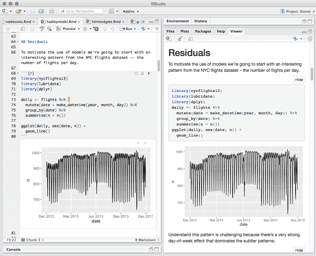
Section 3.2 Notebook
An R Notebook is an R Markdown document with chunks that can be executed independently and interactively, with output visible immediately beneath the input. See Figure 3.5 for an example.
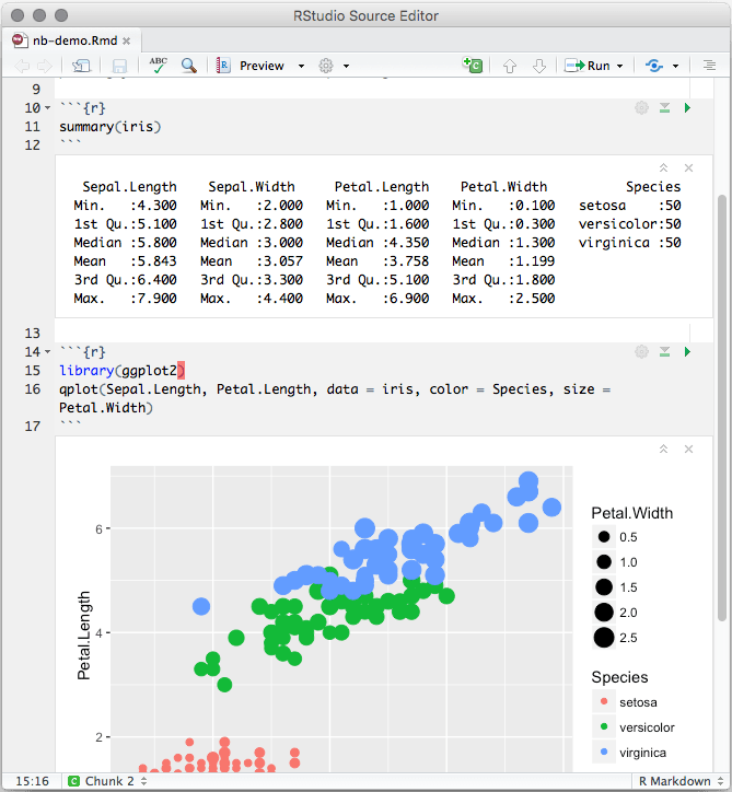
An R Notebook example.
R Notebooks are an implementation of Literate Programming that allows for direct interaction with R while producing a reproducible document with publication-quality output.
Any R Markdown document can be used as a notebook, and all R Notebooks can be rendered to other R Markdown document types. A notebook can therefore be thought of as a special execution mode for R Markdown documents. The immediacy of notebook mode makes it a good choice while authoring the R Markdown document and iterating on code. When you are ready to publish the document, you can share the notebook directly, or render it to a publication format with the
Knit button.
Subsection 3.2.1 Using Notebooks
Subsubsection 3.2.1.1 Creating a Notebook
You can create a new notebook in RStudio with the menu command
File -> New File -> R Notebook, or by using the html_notebook output type in your document’s YAML metadata.
---
title: "My Notebook"
output: html_notebook
---
By default, RStudio enables inline output (Notebook mode) on all R Markdown documents, so you can interact with any R Markdown document as though it were a notebook. If you have a document with which you prefer to use the traditional console method of interaction, you can disable notebook mode by clicking the gear button in the editor toolbar, and choosing
Chunk Output in Console (Figure 3.6).
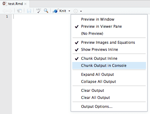
Send the R code chunk output to the console.
If you prefer to use the console by default for all your R Markdown documents (restoring the behavior in previous versions of RStudio), you can make
Chunk Output in Console the default: Tools -> Options -> R Markdown -> Show output inline for all R Markdown documents.
Subsubsection 3.2.1.2 Inserting chunks
Notebook chunks can be inserted quickly using the keyboard shortcut
Ctrl + Alt + I (macOS: Cmd + Option + I), or via the Insert menu in the editor toolbar.
Because all of a chunk’s output appears beneath the chunk (not alongside the statement which emitted the output, as it does in the rendered R Markdown output), it is often helpful to split chunks that produce multiple outputs into two or more chunks which each produce only one output. To do this, select the code to split into a new chunk (Figure 3.7), and use the same keyboard shortcut for inserting a new code chunk (Figure 3.8).
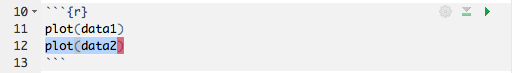
Select the code to split into a new chunk.
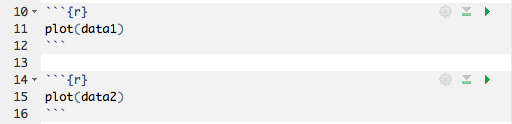
Insert a new chunk from the code selected before.
Subsubsection 3.2.1.3 Executing code
Code in the notebook is executed with the same gestures you would use to execute code in an R Markdown document:
-
Use the green triangle button on the toolbar of a code chunk that has the tooltip "Run Current Chunk", or
Ctrl + Shift + Enter(macOS:Cmd + Shift + Enter) to run the current chunk. -
Press
Ctrl + Enter(macOS:Cmd + Enter) to run just the current statement. Running a single statement is much like running an entire chunk consisting only of that statement. -
There are other ways to run a batch of chunks if you click the menu
Runon the editor toolbar, such asRun All,Run All Chunks Above, andRun All Chunks Below.
The primary difference is that when executing chunks in an R Markdown document, all the code is sent to the console at once, but in a notebook, only one line at a time is sent. This allows execution to stop if a line raises an error. When you execute code in a notebook, an indicator will appear in the gutter to show you execution progress (Figure 3.9). Lines of code that have been sent to R are marked with dark green; lines that have not yet been sent to R are marked with light green. If at least one chunk is waiting to be executed, you will see a progress meter appear in the editor’s status bar, indicating the number of chunks remaining to be executed. You can click on this meter at any time to jump to the currently executing chunk. When a chunk is waiting to execute, the
Run button in its toolbar will change to a "queued" icon. If you do not want the chunk to run, you can click on the icon to remove it from the execution queue.
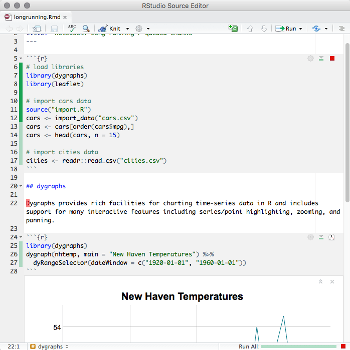
The indicator in the gutter to show the execution progress of a code chunk in the notebook.
In general, when you execute code in a notebook chunk, it will do exactly the same thing as it would if that same code were typed into the console. There are however a few differences:
-
Output: The most obvious difference is that most forms of output produced from a notebook chunk are shown in the chunk output rather than, for example, the RStudio Viewer or the Plots pane. Console output (including warnings and messages) appears both at the console and in the chunk output.
-
Working directory: The current working directory inside a notebook chunk is always the directory containing the notebook
.Rmdfile. This makes it easier to use relative paths inside notebook chunks, and also matches the behavior when knitting, making it easier to write code that works identically both interactively and in a standalone render. You’ll get a warning if you try to change the working directory inside a notebook chunk, and the directory will revert back to the notebook’s directory once the chunk is finished executing. You can suppress this warning by using thewarnings = FALSEchunk option. If it is necessary to execute notebook chunks in a different directory, you can change the working directory for all your chunks by using the knitrroot.diroption. For instance, to execute all notebook chunks in the grandparent folder of the notebook:knitr::opts_knit$set(root.dir = normalizePath("..")). This option is only effective when used inside the setup chunk. Also note that, as in knitr, theroot.dirchunk option applies only to chunks; relative paths in Markdown are still relative to the notebook’s parent folder. -
Warnings: Inside a notebook chunk, warnings are always displayed immediately rather than being held until the end, as in
options(warn = 1). -
Plots: Plots emitted from a chunk are rendered to match the width of the editor at the time the chunk was executed. The height of the plot is determined by the golden ratio. The plot’s display list is saved, too, and the plot is re-rendered to match the editor’s width when the editor is resized.
You can use the
fig.width, fig.height, and fig.asp chunk options to manually specify the size of rendered plots in the notebook; you can also use knitr::opts_chunk$set(fig.width = ..., fig.height = ...) in the setup chunk to to set a default rendered size. Note, however, specifying a chunk size manually suppresses the generation of the display list, so plots with manually specified sizes will be resized using simple image scaling when the notebook editor is resized. To execute an inline R expression in the notebook, put your cursor inside the chunk and press Ctrl + Enter (macOS: Cmd + Enter). As in the execution of ordinary chunks, the content of the expression will be sent to the R console for evaluation. The results will appear in a small pop-up window next to the code (Figure 3.10).
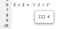
Output from an inline R expression in the notebook.
In notebooks, inline R expressions can only produce text (not figures or other kinds of output). It is also important that inline R expressions executes quickly and do not have side-effects, as they are executed whenever you save the notebook.
Notebooks are typically self-contained. However, in some situations, it is preferable to re-use code from an R script as a notebook chunk, as in knitr’s code externalization. This can be done by using
knitr::read_chunk() in your notebook’s setup chunk, along with a special ## ---- chunkname annotation in the R file from which you intend to read code. Here is a minimal example with two files:
example.Rmd
```{r setup}
knitr::read_chunk("example.R")
```
example.R
## ---- chunk
1 + 1
When you execute the empty chunk in the notebook
example.Rmd, code from the external file example.R will be inserted, and the results displayed inline, as though the chunk contained that code (Figure 3.11).
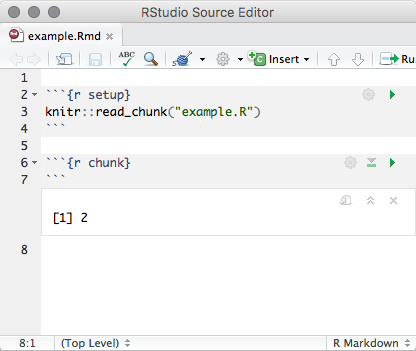
Execute a code chunk read from an external R script.
Subsubsection 3.2.1.4 Chunk output
When code is executed in the notebook, its output appears beneath the code chunk that produced it. You can clear an individual chunk’s output by clicking the
X button in the upper right corner of the output, or collapse it by clicking the chevron.
It is also possible to clear or collapse all of the output in the document at once using the
Collapse All Output and Clear All Output menu items available on the gear menu in the editor toolbar (Figure 3.6).
If you want to fully reset the state of the notebook, the item
Restart R and Clear Output on the Run menu on the editor toolbar will do the job.
Ordinary R Markdown documents are "knitted", but notebooks are "previewed". While the notebook preview looks similar to a rendered R Markdown document, the notebook preview _does not execute any of your R code chunks_. It simply shows you a rendered copy of the Markdown output of your document along with the most recent chunk output. This preview is generated automatically whenever you save the notebook (whether you are viewing it in RStudio or not); see the section beneath on the
*.nb.html file for details.
When
html_notebook is the topmost (default) format in your YAML metadata, you will see a Preview button in the editor toolbar. Clicking it will show you the notebook preview (Figure 3.12).
Preview a notebook.
If you have configured R Markdown previewing to use the Viewer pane (as illustrated in Figure 3.12), the preview will be automatically updated whenever you save your notebook.
When an error occurs while a notebook chunk is executing (Figure 3.13):

Errors in a notebook.
-
Execution will stop; the remaining lines of that chunk (and any chunks that have not yet been run) will not be executed.
-
The editor will scroll to the error.
-
The line of code that caused the error will have a red indicator in the editor’s gutter.
If you want your notebook to keep running after an error, you can suppress the first two behaviors by specifying
error = TRUE in the chunk options. In most cases, it should not be necessary to have the console open while using the notebook, as you can see all of the console output in the notebook itself. To preserve vertical space, the console will be automatically collapsed when you open a notebook or run a chunk in the notebook. If you prefer not to have the console hidden when chunks are executed, uncheck the option from the menu Tools -> Global Options -> R Markdown -> Hide console automatically when executing notebook chunks.
Subsection 3.2.2 Saving and sharing
Subsubsection 3.2.2.1 Notebook file
When a notebook
*.Rmd file is saved, a *.nb.html file is created alongside it. This file is a self-contained HTML file which contains both a rendered copy of the notebook with all current chunk outputs (suitable for display on a website) and a copy of the *.Rmd file itself.
You can view the
*.nb.html file in any ordinary web browser. It can also be opened in RStudio; when you open there (e.g., using File -> Open File), RStudio will do the following:
-
Open the
*.Rmdfile in a new RStudio editor tab. -
Extract the chunk outputs from the
*.nb.htmlfile, and place them appropriately in the editor.
Note that the
*.nb.html file is only created for R Markdown documents that are notebooks (i.e., at least one of their output formats is html_notebook). It is possible to have an R Markdown document that includes inline chunk output beneath code chunks, but does not produce an *.nb.html file, when html_notebook is not specified as an output format for the R Markdown document.
Subsubsection 3.2.2.2 Output storage
The document’s chunk outputs are also stored in an internal RStudio folder beneath the project’s
.Rproj.user folder. If you work with a notebook but do not have a project open, the outputs are stored in the RStudio state folder in your home directory (the location of this folder varies between the desktop and the server).
Subsubsection 3.2.2.3 Version control
One of the major advantages of R Notebooks compared to other notebook systems is that they are plain-text files and therefore work well with version control. We recommend checking in both the
*.Rmd and *.nb.html files into version control, so that both your source code and output are available to collaborators. However, you can choose to include only the *.Rmd file (with a .gitignore that excludes *.nb.html) if you want each collaborator to work with their own private copies of the output.
Subsection 3.2.3 Notebook format
While RStudio provides a set of integrated tools for authoring R Notebooks, the notebook file format itself is decoupled from RStudio. The rmarkdown package provides several functions that can be used to read and write R Notebooks outside of RStudio.
In this section, we describe the internals of the notebook format. It is primarily intended for front-end applications using or embedding R, or other users who are interested in reading and writing documents using the R Notebook format. We recommend that beginners skip this section when reading this book or using notebooks for the first time.
R Notebooks are HTML documents with data written and encoded in such a way that:
-
The source Rmd document can be recovered, and
-
Chunk outputs can be recovered.
To generate an R Notebook, you can use
rmarkdown::render() and specify the html_notebook output format in your document’s YAML metadata. Documents rendered in this form will be generated with the .nb.html file extension, to indicate that they are HTML notebooks.
To ensure chunk outputs can be recovered, the elements of the R Markdown document are enclosed with HTML comments, providing more information on the output. For example, chunk output might be serialized in the form:
<!-- rnb-chunk-begin -->
<!-- rnb-output-begin -->
<pre><code>Hello, World!</code></pre>
<!-- rnb-output-end -->
<!-- rnb-chunk-end -->
Because R Notebooks are just HTML documents, they can be opened and viewed in any web browser; in addition, hosting environments can be configured to recover and open the source Rmd document, and also recover and display chunk outputs as appropriate.
Subsubsection 3.2.3.1 Generating R Notebooks with custom output
It is possible to render an HTML notebook with custom chunk outputs inserted in lieu of the result that would be generated by evaluating the associated R code. This can be useful for front-end editors that show the output of chunk execution inline, or for conversion programs from other notebook formats where output is already available from the source format. To facilitate this, one can provide a custom "output source" to
rmarkdown::render(). Let’s investigate with a simple example:
rmd_stub = "examples/r-notebook-stub.Rmd"
cat(readLines(rmd_stub), sep = "\n")
---
title: "R Notebook Stub"
output: html_notebook
---

```{r chunk-one}
print("Hello, World!")
```
Let’s try to render this document with a custom output source, so that we can inject custom output for the single chunk within the document. The output source function will accept:
-
code: The code within the current chunk. -
context: An environment containing active chunk options and other chunk information. -
...: Optional arguments reserved for future expansion. In particular, thecontextelementslabelandchunk.indexcan be used to help identify which chunk is currently being rendered.
output_source = function(code, context, ...) {
  logo = file.path(R.home("doc"), "html", "logo.jpg")
  if (context$label == "chunk-one") list(
    rmarkdown::html_notebook_output_code("# R Code"),
    paste("Custom output for chunk:", context$chunk.index),
    rmarkdown::html_notebook_output_code("# R Logo"),
    rmarkdown::html_notebook_output_img(logo)
  )
}
output_file = rmarkdown::render(
  rmd_stub,
  output_options = list(output_source = output_source),
  quiet = TRUE
)
We have now generated an R Notebook. Open this document in a web browser, and it will show that the
output_source function has effectively side-stepped evaluation of code within that chunk, and instead returned the injected result.
Subsubsection 3.2.3.2 Implementing output sources
In general, you can provide regular R output in your output source function, but rmarkdown also provides a number of endpoints for insertion of custom HTML content. These are documented within
?html_notebook_output.
Using these functions ensures that you produce an R Notebook that can be opened in R frontends (e.g., RStudio).
Subsubsection 3.2.3.3 Parsing R Notebooks
The
rmarkdown::parse_html_notebook() function provides an interface for recovering and parsing an HTML notebook.
parsed = rmarkdown::parse_html_notebook(output_file)
str(parsed, width = 60, strict.width = 'wrap')
List of 4
$ source : chr [1:300] "<!DOCTYPE html>" "" "<html>" "" ...
$ rmd : chr [1:8] "---" "title: \"R Notebook Stub\""
   "output: html_notebook" "---" ...
$ header : chr [1:180] "<head>" "" "<meta charset=\"utf-8\"
   />" "<meta name=\"generator\" content=\"pandoc\" />" ...
$ annotations:List of 18
..$ :List of 4
.. ..$ row : int 213
.. ..$ label: chr "text"
.. ..$ state: chr "begin"
.. ..$ meta : NULL
..$ :List of 4
.. ..$ row : int 214
.. ..$ label: chr "text"
.. ..$ state: chr "end"
.. ..$ meta : NULL
..$ :List of 4
.. ..$ row : int 215
.. ..$ label: chr "chunk"
.. ..$ state: chr "begin"
.. ..$ meta : NULL
..$ :List of 4
.. ..$ row : int 216
.. ..$ label: chr "output"
.. ..$ state: chr "begin"
.. ..$ meta :List of 1
.. .. ..$ data: chr "\n<!-- rnb-source-begin
   eyJkYXRhIjoiYGBgclxuIyBSIENvZGVcbmBgYCJ9 -->\n\n```r\n#
   R Code\n```\n\n<!-- rnb-source-end -->\n"
..$ :List of 4
.. ..$ row : int 217
.. ..$ label: chr "source"
.. ..$ state: chr "begin"
.. ..$ meta :List of 1
.. .. ..$ data: chr "```r\n# R Code\n```"
..$ :List of 4
.. ..$ row : int 219
.. ..$ label: chr "source"
.. ..$ state: chr "end"
.. ..$ meta : NULL
..$ :List of 4
.. ..$ row : int 220
.. ..$ label: chr "output"
.. ..$ state: chr "end"
.. ..$ meta : NULL
..$ :List of 4
.. ..$ row : int 221
.. ..$ label: chr "output"
.. ..$ state: chr "begin"
.. ..$ meta :List of 1
.. .. ..$ data: chr "Custom output for chunk: 1\n"
..$ :List of 4
.. ..$ row : int 223
.. ..$ label: chr "output"
.. ..$ state: chr "end"
.. ..$ meta : NULL
..$ :List of 4
.. ..$ row : int 224
.. ..$ label: chr "output"
.. ..$ state: chr "begin"
.. ..$ meta :List of 1
.. .. ..$ data: chr "\n<!-- rnb-source-begin
   eyJkYXRhIjoiYGBgclxuIyBSIExvZ29cbmBgYCJ9 -->\n\n```r\n#
   R Logo\n```\n\n<!-- rnb-source-end -->\n"
..$ :List of 4
.. ..$ row : int 225
.. ..$ label: chr "source"
.. ..$ state: chr "begin"
.. ..$ meta :List of 1
.. .. ..$ data: chr "```r\n# R Logo\n```"
..$ :List of 4
.. ..$ row : int 227
.. ..$ label: chr "source"
.. ..$ state: chr "end"
.. ..$ meta : NULL
..$ :List of 4
.. ..$ row : int 228
.. ..$ label: chr "output"
.. ..$ state: chr "end"
.. ..$ meta : NULL
..$ :List of 4
.. ..$ row : int 229
.. ..$ label: chr "output"
.. ..$ state: chr "begin"
.. ..$ meta :List of 1
.. .. ..$ data: chr "\n<!-- rnb-plot-begin -->\n\n<img
   src=\"data:image/png;base64,/9j/4QSfRXhpZgAATU0AKgAAAA"..
   __truncated__
..$ :List of 4
.. ..$ row : int 230
.. ..$ label: chr "plot"
.. ..$ state: chr "begin"
.. ..$ meta : NULL
..$ :List of 4
.. ..$ row : int 232
.. ..$ label: chr "plot"
.. ..$ state: chr "end"
.. ..$ meta : NULL
..$ :List of 4
.. ..$ row : int 233
.. ..$ label: chr "output"
.. ..$ state: chr "end"
.. ..$ meta : NULL
..$ :List of 4
.. ..$ row : int 234
.. ..$ label: chr "chunk"
.. ..$ state: chr "end"
.. ..$ meta : NULL
This interface can be used to recover the original Rmd source, and also (with some more effort from the front-end) the ability to recover chunk outputs from the document itself.
Section 3.3 PDF document
To create a PDF document from R Markdown, you specify the
pdf_document output format in the YAML metadata:
---
title: "Habits"
author: John Doe
date: March 22, 2005
output: pdf_document
---
Within R Markdown documents that generate PDF output, you can use raw LaTeX, and even define LaTeX macros. See Pandoc’s documentation on the raw_tex extension for details.
Subsection 3.3.1 Table of contents
You can add a table of contents using the
toc option and specify the depth of headers that it applies to using the toc_depth option. For example:
---
title: "Habits"
output:
  pdf_document:
    toc: true
    toc_depth: 2
---
If the TOC depth is not explicitly specified, it defaults to 2 (meaning that all level 1 and 2 headers will be included in the TOC), while it defaults to 3 in
html_document.
You can add section numbering to headers using the
number_sections option:
---
title: "Habits"
output:
  pdf_document:
    toc: true
    number_sections: true
---
If you are familiar with LaTeX,
number_sections: true means \section{}, and number_sections: false means \section*{} for sections in LaTeX (it also applies to other levels of "sections" such as \chapter{}, and \subsection{}).
Subsection 3.3.2 Figure options
There are a number of options that affect the output of figures within PDF documents:
-
fig_widthandfig_heightcan be used to control the default figure width and height (6.5x4.5 is used by default). -
fig_cropcontrols whether thepdfcroputility, if available in your system, is automatically applied to PDF figures (this istrueby default). -
If you are using TinyTeX as your LaTeX distribution, we recommend that you run
tinytex::tlmgr_install("pdfcrop")to install the LaTeX packagepdfcrop. You also have to make sure the system package ghostscript is available in your system forpdfcropto work. For macOS users who have installed Homebrew,ghostscriptcan be installed viabrew install ghostscript. -
If your graphics device is
postscript, we recommend that you disable this feature (see more info in the knitr issue #1365).
---
title: "Habits"
output:
  pdf_document:
    fig_width: 7
    fig_height: 6
    fig_caption: true
---
Subsection 3.3.3 Data frame printing
You can enhance the default display of data frames via the
df_print option. Valid values are presented in Table 3.14.
df_print option for the pdf_document format| Option | Description |
|---|---|
default |
Call the print.data.frame generic method |
kable |
Use the knitr::kable() function |
tibble |
Use the tibble::print.tbl_df() function |
| A custom function | Use the function to create the table. See Subsubsection 3.1.6.2. |
For example:
---
title: "Habits"
output:
  pdf_document:
    df_print: kable
---
Subsection 3.3.4 Syntax highlighting
The
highlight option specifies the syntax highlighting style. Its usage in pdf_document is the same as html_document (Subsection 4.1.3). For example:
---
title: "Habits"
output:
  pdf_document:
    highlight: tango
---
Subsection 3.3.5 LaTeX options
Many aspects of the LaTeX template used to create PDF documents can be customized using _top-level_ YAML metadata (note that these options do not appear underneath the
output section, but rather appear at the top level along with title, author, and so on). For example:
---
title: "Crop Analysis Q3 2013"
output: pdf_document
fontsize: 11pt
geometry: margin=1in
---
A few available metadata variables are displayed in Table 3.15 (consult the Pandoc manual for the full list):
| Variable | Description |
|---|---|
lang |
Document language code |
fontsize |
Font size (e.g., 10pt, 11pt, or 12pt) |
documentclass |
LaTeX document class (e.g., article) |
classoption |
Options for documentclass (e.g., oneside) |
geometry |
Options for geometry class (e.g., margin=1in) |
mainfont, sansfont, monofont, mathfont
|
Document fonts (works only with xelatex and lualatex) |
linkcolor, urlcolor, citecolor
|
Color for internal, external, and citation links |
Subsection 3.3.6 LaTeX packages for citations
By default, citations are processed through
pandoc-citeproc, which works for all output formats. For PDF output, sometimes it is better to use LaTeX packages to process citations, such as natbib or biblatex. To use one of these packages, just set the option citation_package to be natbib or biblatex, e.g.
---
output:
  pdf_document:
    citation_package: natbib
---
Subsection 3.3.7 Advanced customization
Subsubsection 3.3.7.1 LaTeX engine
By default, PDF documents are rendered using
pdflatex. You can specify an alternate engine using the latex_engine option. Available engines are pdflatex, xelatex, and lualatex. For example:
---
title: "Habits"
output:
  pdf_document:
    latex_engine: xelatex
---
The main reasons you may want to use
xelatex or lualatex are: (1) They support Unicode better; (2) It is easier to make use of system fonts. See some posts on Stack Overflow for more detailed explanations, e.g., https://tex.stackexchange.com/q/3393/9128 and https://tex.stackexchange.com/q/36/9128.
Subsubsection 3.3.7.2 Keeping intermediate TeX
R Markdown documents are converted to PDF by first converting to a TeX file and then calling the LaTeX engine to convert to PDF. By default, this TeX file is removed, however if you want to keep it (e.g., for an article submission), you can specify the
keep_tex option. For example:
---
title: "Habits"
output:
  pdf_document:
    keep_tex: true
---
Subsubsection 3.3.7.3 Includes
You can do more advanced customization of PDF output by including additional LaTeX directives and/or content or by replacing the core Pandoc template entirely. To include content in the document header or before/after the document body, you use the
includes option as follows:
---
title: "Habits"
output:
  pdf_document:
    includes:
      in_header: preamble.tex
      before_body: doc-prefix.tex
      after_body: doc-suffix.tex
---
Subsubsection 3.3.7.4 Custom templates
You can also replace the underlying Pandoc template using the
template option:
---
title: "Habits"
output:
  pdf_document:
    template: quarterly-report.tex
---
Consult the documentation on Pandoc templates for additional details on templates. You can also study the default LaTeX template as an example.
Subsection 3.3.8 Other features
Similar to HTML documents, you can enable or disable certain Markdown extensions for generating PDF documents. See Subsubsection 3.1.10.4 for details. You can also pass more custom Pandoc arguments through the
pandoc_args option (Subsubsection 3.1.10.5), and define shared options in _output.yml (Subsection 3.1.11).
Section 3.4 Word document
To create a Word document from R Markdown, you specify the
word_document output format in the YAML metadata of your document:
---
title: "Habits"
author: John Doe
date: March 22, 2005
output: word_document
---
The most notable feature of Word documents is the Word template, which is also known as the "style reference document". You can specify a document to be used as a style reference in producing a
*.docx file (a Word document). This will allow you to customize things such as margins and other formatting characteristics. For best results, the reference document should be a modified version of a .docx file produced using rmarkdown or Pandoc. The path of such a document can be passed to the reference_docx argument of the word_document format. Pass "default" to use the default styles. For example:
---
title: "Habits"
output:
  word_document:
    reference_docx: my-styles.docx
---
For more on how to create and use a reference document, you may watch this short video:
https://vimeo.com/110804387, or read this detailed article: https://rmarkdown.rstudio.com/articles_docx.html.
Subsection 3.4.1 Other features
Refer to Section 3.1 for the documentation of most features of Word documents, including figure options (Subsection 3.1.5), data frame printing (Subsection 3.1.6), syntax highlighting (Subsection 4.1.3), keeping Markdown (Subsubsection 3.1.10.1), Markdown extensions (Subsubsection 3.1.10.4), Pandoc arguments (Subsubsection 3.1.10.5), and shared options (Subsection 3.1.11).
Section 3.5 OpenDocument Text document
To create an OpenDocument Text (ODT) document from R Markdown, you specify the
odt_document output format in the YAML metadata of your document:
---
title: "Habits"
author: John Doe
date: March 22, 2005
output: odt_document
---
Similar to
word_document, you can also provide a style reference document to odt_document through the reference_odt option. For best results, the reference ODT document should be a modified version of an ODT file produced using rmarkdown or Pandoc. For example:
---
title: "Habits"
output:
  odt_document:
    reference_odt: my-styles.odt
---
Subsection 3.5.1 Other features
Refer to Section 3.1 for the documentation of most features of ODT documents, including figure options (Subsection 3.1.5), keeping Markdown (Subsubsection 3.1.10.1), header and before/after body inclusions (Subsubsection 3.1.10.2), custom templates (Subsubsection 3.1.10.3), Markdown extensions (Subsubsection 3.1.10.4), Pandoc arguments (Subsubsection 3.1.10.5), and shared options (Subsection 3.1.11).
Section 3.6 Rich Text Format document
To create a Rich Text Format (RTF) document from R Markdown, you specify the
rtf_document output format in the YAML metadata of your document:
---
title: "Habits"
author: John Doe
date: March 22, 2005
output: rtf_document
---
If you know the RTF format really well, you can actually embed raw RTF content in R Markdown. For example, you may create a table in RTF using other software packages, and insert it to your final RTF output document. An RTF document is essentially a plain-text document, so you can read it into R using functions like
readLines(). Now suppose you have an RTF table in the file table.rtf. To embed it in R Markdown, you read it and pass to knitr::raw_output(), e.g.,
```{r, echo=FALSE}
knitr::raw_output(readLines('table.rtf'))
```
Subsection 3.6.1 Other features
Refer to Section 3.1 for the documentation of most features of RTF documents, including table of contents (Subsection 3.1.1), figure options (Subsection 3.1.5), keeping Markdown (Subsubsection 3.1.10.1), Markdown extensions (Subsubsection 3.1.10.4), Pandoc arguments (Subsubsection 3.1.10.5), and shared options (Subsection 3.1.11).
Section 3.7 Markdown document
In some cases, you might want to produce plain Markdown output from R Markdown (e.g., to create a document for a system that accepts Markdown input like Stack Overflow).
To create a Markdown document from R Markdown, you specify the
md_document output format in the front-matter of your document:
---
title: "Habits"
author: John Doe
date: March 22, 2005
output: md_document
---
Subsection 3.7.1 Markdown variants
By default, the
md_document format produces "strict" Markdown (i.e., conforming to the original Markdown specification with no extensions). You can generate a different flavor of Markdown using the variant option. For example:
---
output:
  md_document:
    variant: markdown_github
---
Valid values are:
-
markdown(Full Pandoc Markdown) -
markdown_strict(Original Markdown specification; the default) -
markdown_github(GitHub Flavored Markdown) -
markdown_mmd(MultiMarkdown) -
markdown_phpextra(PHP Markdown extra) You can also compose custom Markdown variants. For example:
---
output:
  md_document:
    variant: markdown_strict+backtick_code_blocks+autolink_bare_uris
---
See Pandoc’s Manual for all of the Markdown extensions and their names to be used in composing custom variants.
Subsubsection 3.7.1.1 Publishing formats
Many popular publishing systems now accept Markdown as input. Table 3.16 shows the correct Markdown variants to use for some popular systems.
| System | Markdown Variant |
|---|---|
| GitHub Wikis | markdown_github |
| Drupal | markdown_phpextra |
| WordPress.com | markdown_phpextra+backtick_code_blocks |
| StackOverflow | markdown_strict+autolink_bare_uris |
In many cases, you can simply copy and paste the Markdown generated by
rmarkdown::render() into the editing interface of the system you are targeting. Note, however, that if you have embedded plots or other images, you will need to upload them separately and fix up their URLs to point to the uploaded location. If you intend to build websites based on R Markdown, we recommend that you use the more straightforward solutions such as blogdown [7] [10] as introduced in Chapter 10 instead of manually copying the Markdown content.
Subsection 3.7.2 Other features
Refer to Section 3.1 for the documentation of other features of Markdown documents, including table of contents (Subsection 3.1.1), figure options (Subsection 3.1.5), header and before/after body inclusions (Subsubsection 3.1.10.2), Pandoc arguments (Subsubsection 3.1.10.5), and shared options (Subsection 3.1.11).
Section 3.8 R package vignette
The
html_vignette format provides a lightweight alternative to html_document suitable for inclusion in packages to be released to CRAN. It reduces the size of a basic vignette from 600Kb to around 10Kb. The format differs from a conventional HTML document as follows:
-
Never uses retina figures
-
Has a smaller default figure size
-
Uses a custom lightweight CSS stylesheet
To use
html_vignette, you specify it as the output format and add some additional vignette related settings via the \Vignette*{} macros:
---
title: "Your Vignette Title"
output: rmarkdown::html_vignette
vignette: >
  %\VignetteEngine{knitr::rmarkdown}
  %\VignetteIndexEntry{Your Vignette Title}
  %\VignetteEncoding{UTF-8}
---
Note that you should change the
title field and the \VignetteIndexEntry{} to match the title of your vignette.
Most options for
html_document (Section 3.1) also work for html_vignette, except fig_retina and theme, which have been set to null internally in this format.
The
html_vignette template includes a basic CSS theme. To override this theme, you can specify your own CSS in the document metadata as follows:
output:
  rmarkdown::html_vignette:
    css: mystyles.css
The default figure size is 3x3. Because the figure width is small, usually you will be able to put two images side-by-side if you set the chunk option
fig.show='hold', e.g.,
```{r, fig.show='hold'}
plot(1:10)
plot(10:1)
```
If you want larger figure sizes you can change the
fig_width and fig_height in the document output options or alternatively override the default options on a per-chunk basis.
