Introduction to Data Science Version 3

We can use an example to show how to use linear regression on real data. The example concerns attendances at Australian Rules Football matches. For those in the U.S., Australian Rules Football is closer to what you think of as rugby and not so much like American football. The data in this example concerns matches/ games at the largest stadium for the sport, the Melbourne Cricket Ground (note: Australian Rules football is a winter sport, cricket is a summer sport). The Melbourne Cricket Ground or MCG is also considered the most prestigious ground to play a football match, due to its long association with Australian Rules Football.

Australian Rules Football is the most popular sport to have been developed in Australia. The object is to kick the ball through the larger goal posts, scoring six points. If the ball is touched before it crosses the line under the large posts, or instead passes through the smaller posts on either side of the large goal posts, a single point is scored. The rules ensure that possession of the ball is always changing. There is full body tackling and possession is turned over frequently. This leads to continuous and exciting on-field action.

The main stronghold of Australian Rules Football is in the state of Victoria (south eastern Australia), where the original league, the VFL, became the AFL after its league of mostly Melbourne suburban teams added teams to represent areas outside Victoria, such as West Coast (Perth, the capital of the state of Western Australia) and Adelaide (capital of the state of South Australia). Note that Melbourne is the capital city of Victoria. Much of the popularity of the VFL was based on the rivalries between neighboring suburbs, and teams with long histories, like the Collingwood Football Club - based in one of Melbourne’s most working class suburbs – have large and loyal fan bases.

While it isn’t necessary to know anything about how the sport is played to understand the example, it is useful to know that the Australian Football League, the premiere organization playing Australian Rules Football, was formerly the Victorian Football League, and although teams from outside the Australian state of Victoria have joined, more than half the teams in the league are Victorian, even though Victoria is only one of six Australian states.

The data are available from OzDasl, a website which provides public domain data sets for analysis, and the MCG attendance data has its own page at http://www.statsci.org/data/oz/afl.html.

The variable of interest is MCG attendance, and named ‘MCG’ in the dataset. Most statisticians would refer to this variable as the dependent variable, because it is the variable that we are most interested in predicting: It is the "outcome" of the situation we are trying to understand. Potential explanatory, or independent, variables include club membership, weather on match day, date of match, etc. There is a detailed description of each of the variables available on the website. You can use the data set to test your own theories of what makes football fans decide whether or not to go to a game, but to learn some of the skills we will test a couple of those factors together.

Before we can start, we need R to be able to find the data. Make sure that you download the data to the spot on your computer that R considers the "working" directory. Use this command to find out what the current working directory is:

getwd()

After downloading the data set from OzDasl into your R working directory, read the data set into R as follows:

attend <- read.delim("afl.txt", header=TRUE)
attach(attend)

We include the optional header = TRUE to designate the first row as the column names, and the attach commands turns each of the named columns into a single column vector.

Once we’ve read the data into R, we can examine some plots of the data. With many techniques in data science, it can be quite valuable to visualize the data before undertaking a more detailed analysis. One of the variables we might consider is the combined membership of the two teams playing, a proxy for the popularity of the teams playing.

plot(MCG ~ Members,
  xlab="Combined membership of teams playing",
  ylab="MCG Match Day Attendance")

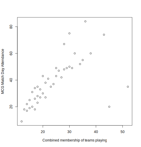
We see evidence of a trend in the points on the left hand side of the graph, and a small group of points representing games with very high combined membership but that don’t seem to fit the trend applying to the rest of data. If it wasn’t for the four "outliers" on the right hand side of the plot, we would be left with a plot showing a very strong relationship.