Section 15.2 Data Formats and Importing Data
The first and easiest strategy for getting data into R is to use the data import dialog in R-Studio. In the upper right hand pane of R-Studio, the “Workspace” tab gives views of currently available data objects, but also has a set of buttons at the top for managing the work space. One of the choices there is the “Import Dataset” button: This enables a drop down menu where one choice is to import, “From Text File...” If you click this option and choose an appropriate file you will get a screen like this:
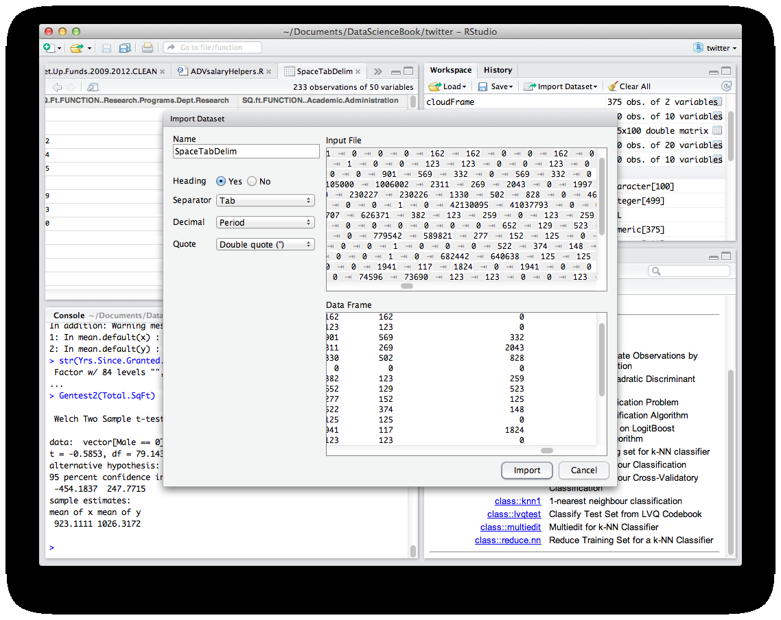
The most important stuff is on the left side. Heading controls whether or not the first line of the text file is treated as containing variable names. The separator drop down gives a choice of different characters that separate the fields/columns in the data. R-Studio tries to guess the appropriate choice here based on a scan of the data. In this case it guessed right by choosing “tab-delimited.” As mentioned above, tab-delimited and comma-delimited are the two most common formats used for interchange between data programs.The next drop down is for “Decimal” and this option accounts for the fact the a dot is used in the U.S. while a comma may be used for the decimal point in Europe and elsewhere. Finally, the “Quote” drop down controls which character is used to contain quoted string/text data. The most common method is double quotes.
Of course, we skipped ahead a bit here because we assumed that an appropriate file of data was available. It might be useful to see some examples of human readable data:
Name, Age, Gender
“Fred”,22,“M”
“Ginger”,21,“F”
The above is a very simple example of a comma delimited file where the first row contains a “header,” i.e. the information about the names of variables. The second and subsequent rows contain actual data. Each field is separated by a comma, and the text strings are enclosed in double quotes. The same file tab-delimited might look like this:
NameAgeGender
“Fred”22“M”
“Ginger”21“F”
Of course you can’t see the tab characters on the screen, but there is one tab character in between each pair of values. In each case, for both comma- and tab-delimited, one line equals one row. The end of a line is marked, invisibly, with a so called “newline” character. On occasion you may run into differences between different operating systems on how this end of line designation is encoded.
Files containing comma or tab delimited data are ubiquitous across the Internet, but sometimes we would like to gain direct access to binary files in other formats. There are a variety of packages that one might use to access binary data. A comprehensive access list appears here:
This page shows a range of methods for obtaining data from a wide variety of programs and formats. Because Excel is such a widely used program for small, informal data sets, we will use it as an example here to illustrate both the power and the pitfalls of accessing binary data with R. Down near the bottom of the page mentioned just above there are several paragraphs of discussion of how to access Excel files with R. In fact, the first sentence mentions that one of the most commonly asked data questions about R is how to access Excel data.
Interestingly, this is one area where Mac and Linux users are at a disadvantage relative to Windows users. This is perhaps because Excel is a Microsoft product, originally written to be native to Windows, and as a result it is easier to create tools that work with Windows. One example noted here is the package called RODBC. The acronym ODBC stands for Open Database Connection, and this is a Windows facility for exchanging data among Windows programs. Although there is a proprietary ODBC driver available for the Mac, most Mac users will want to try a different method for getting access to Excel data.
Another Windows-only package for R is called xlsReadWrite. This package provides convenient one-command calls for importing data directly from Excel spreadsheets or exporting it directly to spreadsheets. There are also more detailed commands that allow manipulating individual cells.
Two additional packages, xlsx and XLConnect, supposedly will work with the Mac, but at the time of this writing both of these packages had version incompatibilities that made it impossible to install the packages directly into R. Note that the vast majority of packages provide the raw “source code” and so it is theoretically possible, but generally highly time consuming, to “compile” your own copies of these packages to create your own installation.
Fortunately, a general purpose data manipulation package called gdata provides essential facilities for importing spreadsheet files. In the example that follows, we will use a function from gdata to read Excel data directly from a website. The gdata package is a kind of “Swiss Army Knife” package containing many different functions for accessing and manipulating data. For example, you may recall that R uses the value “NA” to represent missing data. Frequently, however, it is the case that data sets contain other values, such as 999, to represent missing data. The gdata package has several functions that find and transform these values to be consistent with R’s strategy for handling missing data.
Begin by using install.package() and
library() functions to prepare the gdata package for use:
install.packages("gdata")
# ... lots of output here
library("gdata")
gdata: read.xls support for ‘XLS’ (Excel 97-2004) files
gdata: ENABLED.
gdata: read.xls support for ‘XLSX’ (Excel 2007+) files ENABLED.
Of course, you could also use the EnsurePackage() function that we developed in an earlier chapter, but it was important here to see the output from the
library() function. Note that the gdata package reported some diagnostics about the different versions of Excel data that it supports. Note that this is one of the major drawbacks of binary data formats, particularly proprietary ones: you have to make sure that you have the right software to access the different versions of data that you might encounter. In this case it looks like we are covered for the early versions of Excel (97-2004) as well as later versions of Excel (2007+). We must always be on the lookout, however, for data that is stored in even newer versions of Excel that may not be supported by gdata or other packages.
Now that gdata is installed, we can use the
read.xls() function that it provides. The documentation for the gdata package and the read.xls() function is located here:
A review of the documentation reveals that the only required argument to this function is the location of the XLS file, and that this location can be a pathname, a web location with http, or an Internet location with ftp (file transfer protocol, a way of sending and receiving files without using a web browser). If you hearken back to a very early chapter in this book, you may remember that we accessed some census data that had population counts for all the different U.S. states. For this example, we are going to read the Excel file containing that data directly into a dataframe using the
read.xls() function:
testFrame<-read.xls( + "http://www.census.gov/popest/data/state/totals/2011/tables/NST-EST2011-01.xls")
trying URL ‘http://www.census.gov/popest/data/state/totals/2011/tables/NST-EST2011-01.xls’
Content type ‘application/vnd.ms-excel’ length 31232 bytes (30 Kb)
opened URL
==================================================
downloaded 30 Kb
The command in the first three lines above provides the URL of the Excel file to the
read.xls() function. The subsequent lines of output show the function attempting to open the URL, succeeding, and downloading 30 kilobytes of data.
Next, let’s take a look at what we got back. In R-Studio we can click on the name of the dataframe in the upper right hand data pane or we can use this command:
View(testFrame)
Either method will show the contents of the dataframe in the upper left hand window of R-Studio. Alternatively, we could use the str() function to create a summary of the structure of testFrame:
str(testFrame)
‘data.frame’:65 obs. of  10 variables:
'data.frame': 65 obs. of 10 variables:
$
table.with.row.headers.in.column.A.and.column.hea
ders.in.rows.3.through.4...leading.dots.indicate.
sub.parts.: Factor w/ 65 levels "",".Alabama",..:
62 53 1 64 55 54 60 65 2 3 ...
$ X
: Factor w/ 60 levels "","1,052,567",..: 1 59 60
27 38 47 10 49 32 50 ...
$ X.1
: Factor w/ 59 levels "","1,052,567",..: 1 1 59
27 38 47 10 49 32 50 ...
$ X.2
: Factor w/ 60 levels "","1,052,528",..: 1 60 21
28 39 48 10 51 33 50 ...
$ X.3
: Factor w/ 59 levels "","1,051,302",..: 1 1 21
28 38 48 10 50 33 51 ...
$ X.4
: logi NA NA NA NA NA NA ...
$ X.5
: logi NA NA NA NA NA NA ...
$ X.6
: logi NA NA NA NA NA NA ...
$ X.7
: logi NA NA NA NA NA NA ...
$ X.8
: logi NA NA NA NA NA NA ...
: logi NA NA NA NA NA NA ...
The last few lines are reminiscent of that late 60s song entitled, ““Na Na Hey Hey Kiss Him Goodbye.” Setting aside all the NA NA NA NAs, however, the overall structure is 65 observations of 10 variables, signifying that the spreadsheet contained 65 rows and 10 columns of data. The variable names that follow are pretty bizarre. The first variable name is:
“table.with.row.headers.in.column.A.and.column.headers.in.rows.3.through.4...leading.dots.indicate.sub.parts.”
What a mess! It is clear that
read.xls() treated the upper leftmost cell as a variable label, but was flummoxed by the fact that this was really just a note to human users of the spreadsheet (the variable labels, such as they are, came on lower rows of the spreadsheet). Subsequent variable names include X, X.1, and X.2: clearly the read.xls() function did not have an easy time getting the variable names out of this file.
The other worrisome finding from str() is that all of our data are “factors.” This indicates that R did not see the incoming data as numbers, but rather as character strings that it interpreted as factor data. Again, this is a side effect of the fact that some of the first cells that
read.xls() encountered were text rather than numeric. The numbers came much later in the sheet. This also underscores the idea that it is much better to export a data set in a more regular, structured format such as CSV rather than in the original spreadsheet format. Clearly we have some work to do if we are to make use of these data as numeric population values.
First, we will use an easy trick to get rid of stuff we don’t need. The Census bureau put in three header rows that we can eliminate like this:
testFrame<-testFrame[-1:-3,]
The minus sign used inside the square brackets refers to the index of rows that should be eliminated from the dataframe. So the notation -1:-3 gets rid of the first three rows. We also leave the column designator empty so that we can keep all columns for now. So the interpretation of all of the notation within the square brackets is that rows 1 through 3 should be dropped, all other rows should be included, and all columns should be included. We assign the result back to the same data object thereby replacing the original with our new, smaller, cleaner version.
Next, we know that of the ten variables we got from
read.xls(), only the first five are useful to us (the last five seem to be blank). So this command keeps the first five columns of the dataframe:
testFrame<-testFrame[,1:5]
In the same vein, the tail() function shows us that the last few rows just contained some census bureau notes:
tail(testFrame,5)
So we can safely eliminate those like this:
testFrame<-testFrame[-58:-62,]
If you’re alert you will notice that we could have combined some of these commands, but for the sake of clarity we have done each operation individually. The result (which you can check in the upper right hand pane of R-Studio) is a dataframe with 57 rows and five observations. Now we are ready to perform a couple of data transformations. Before we start these, let’s give our first column a more reasonable name:
testFrame$region <- testFrame[,1]
We’ve used a little hack here to avoid typing out the ridiculously long name of that first variable/column. We’ve used the column notation in the square brackets on the right hand side of the expression to refer to the first column (the one with the ridiculous name) and simply copied the data into a new column entitled “region.” Let’s also remove the offending column with the stupid name so that it does not cause us problems later on:
testFrame<-testFrame[,-1]
Next, we can change formats and data types as needed. We can remove the dots from in front of the state names very easily with
str_replace():
testFrame$region <- str_replace(
+                        testFrame$region,“\.”,“”)
Don’t forget that
str_replace() is part of the stringr package, and you will have to use install.packages() and library() to load it if it is not already in place. The two backslashes in the string expression above are called “escape characters” and they force the dot that follows to be treated as a literal dot rather than as a wildcard character. The dot on its own is a wildcard that matches one instance of any character.
Next, we can use
str_replace_all() and as.numeric() to convert the data contained in the population columns to usable numbers. Remember that those columns are now represented as R “factors” and what we are doing is taking apart the factor labels (which are basically character strings that look like this: “308,745,538”) and making them into numbers. This is sufficiently repetitive that we could probably benefit by created our own function call to do it:
#
This function is flexible in that it will deal with both unwanted commas and spaces, and will convert strings into numbers whether they are integers or not (i.e., possibly with digits after the decimal point). So we can now run this a few times to create new vectors on the dataframe that contain the numeric values we wanted:
testFrame$april10census <-Numberize(testFrame$X)
testFrame$april10base <-Numberize(testFrame$X.1)
testFrame$july10pop <-Numberize(testFrame$X.2)
testFrame$july11pop <-Numberize(testFrame$X.3)
By the way, the choice of variable names for the new columns in the dataframe was based on an examination of the original data set that was imported by
read.xls(). You can (and should) confirm that the new columns on the dataframe are numeric. You can use str() to accomplish this.
We’ve spent half a chapter so far just looking at one method of importing data from an external file (either on the web or local storage). A lot of our time was spent conditioning the data we got in order to make it usable for later analysis. Herein lies a very important lesson (or perhaps two). An important, and sometimes time consuming aspect of what data scientists do is to make sure that data are “fit for the purpose” to which they are going to be put. We had the convenience of importing a nice data set directly from the web with one simple command, and yet getting those data actually ready to analyze took several additional steps.
A related lesson is that it is important and valuable to try to automate as many of these steps as possible. So when we saw that numbers had gotten stored as factor labels, we moved immediately to create a general function that would convert these to numbers. Not only does this save a lot of future typing, it prevents mistakes from creeping into our processes.

