Introduction to Data Science Version 3

Let’s begin by talking a little bit about association rules. Take a look at the figure with all of the boxes and arrows.

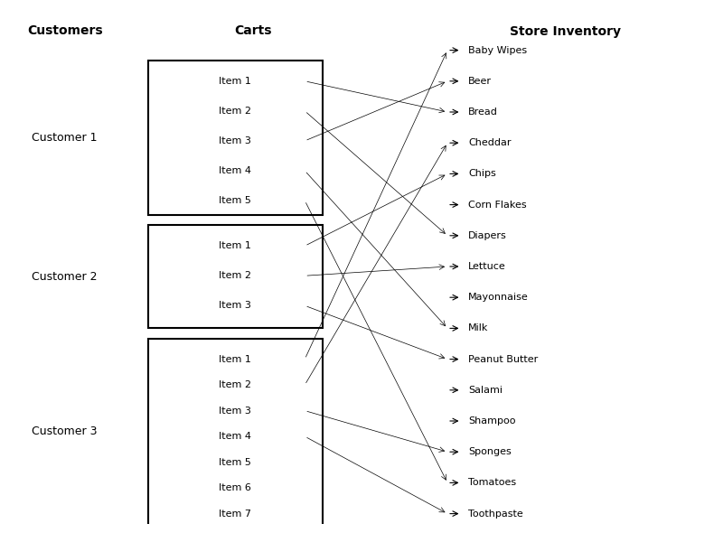
From the figure you can see that each supermarket customer has a grocery cart that contains several items from the larger set of items that the grocery store stocks. The association rules algorithm (also sometimes called affinity analysis) tries out many different propositions, such as "if diapers are purchased, then beer is also purchased." The algorithm uses a dataset of transactions (in the example above, these are the individual carts) to evaluate a long list of these rules for a value called "support." Support is the proportion of times that a particular pairing occurs across all shopping carts. The algorithm also evaluates another quantity called "confidence", which is how frequently a particular pair occurs among all the times when the first item is present. If you look back at the figure again, we had support of 0.67 (the diapers-beer association occurred in two out of the three carts) and confidence of 1.0 ("beer" occurred 100% of the time with "diapers"). In practice, both support and confidence are generally much lower than in this example, but even a rule with low support and smallish confidence might reveal purchasing patterns that grocery store managers could use to guide pricing, coupon offers, or advertising strategies.

We can get started with association rules mining very easily using the R package known as "arules." In R-Studio, you can get the arules package ready using the following commands:

install.packages("arules")
library(arules)

We will begin our exploration of association rules mining using a dataset that is built into the arules package. For the sake of familiarity, we will use the Groceries dataset. Note that by using the Groceries data set, we have relieved ourselves of the burden of data preparation, as the authors of the arules package have generously made sure that Groceries is ready to be analyzed. So we are skipping right to Step 2 in our four step process - exploratory data analysis. You can make the Groceries data set ready with this command:

data(Groceries)

Next, lets run the summary() function on Groceries so that we can see what is in there:

summary(Groceries)

transactions as itemMatrix in sparse format with
 9835 rows (elements/itemsets/transactions) and
 169 columns (items) and a density of 0.02609146

most frequent items:

soda      whole milk   other vegetables   rolls/buns
1715            2513               1903         1809

yogurt       (Other)
  1372         34055

element (itemset/transaction) length distribution:

sizes
  1 2 3 4 5 6 7 8 9 10
11 12 13 14 15 16
2159 1643 1299 1005 855 645 545 438 350 246
182 117 78 77 55 46
17 18 19 20 21 22 23 24 26 27
28 29 32
29 14 14 9 11 4 6 1 1 1
1 3 1

 Min.   1st Qu.   Median   Mean  3rd Qu.    Max.
1.000     2.000    3.000  4.409    6.000  32.000

includes extended item information - examples:
       labels  level2           level1
1 frankfurter sausage meet and sausage
2     sausage sausage meet and sausage
3  liver loaf sausage meet and sausage

Right after the summary command line we see that Groceries is an itemMatrix object in sparse format. So what we have is a nice, rectangular data structure with 9835 rows and 169 columns, where each row is a list of items that might appear in a grocery cart. The word "matrix" in this case, is just referring to this rectangular data structure. The columns are the individual items. A little later in the output we see that there are 169 columns, which means that there are 169 items. The reason the matrix is called "sparse" is that very few of these items exist in any given grocery basket. By the way, when an item appears in a basket, its cell contains a one, while if an item is not in a basket, its cell contains a zero. So in any given row, most of the cells are zero and very few are one and this is what is meant by sparse. We can see from the Min, Median, Mean, and Max output that every cart has at least one item, half the carts have more than three items, the average number of items in a cart is 4.4 and the maximum number of items in a cart is 32.

The output also shows us which items occur in grocery baskets most frequently. If you like working with spreadsheets, you could imagine going to the very bottom of the column that is marked "whole milk" and putting in a formula to sum up all of the ones in that column. You would come up with 2513, indicating that there are 2513 grocery baskets that contain whole milk. Remember that every row/basket that has a one in the whole milk column has whole milk in that basket, whereas a zero would appear if the basket did not contain whole milk. You might wonder what the data field would look like if a grocery cart contained two gallons of whole milk. For the present data mining exercise we can ignore that problem by assuming that any non-zero amount of whole milk is represented by a one. Other data mining techniques could take advantage of knowing the exact amount of a product, but association rules does not need to know that amount - just whether the product is present or absent.

Another way of inspecting our sparse matrix is with the itemFrequencyPlot() function. This produces a bar graph that is similar in concept to a histogram: it shows the relative frequency of occurrence of different items in the matrix. When using the itemFrequencyPlot() function, you must specify the minimum level of "support" needed to include an item in the plot. Remember the mention of support earlier in the chapter - in this case it simply refers to the relative frequency of occurrence of something. We can make a guess as to what level of support to choose based on the results of the summary() function we ran earlier in the chapter. For example, the item "yogurt" appeared in 1372 out of 9835 rows or about 14% of cases. So we can set the support parameter to somewhere around 10%-15% in order to get a manageable number of items:

itemFrequencyPlot(Groceries,support=0.1)

This command produces the following plot:

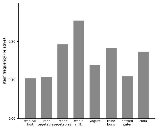
We can see that yogurt is right around 14% as expected and we also see a few other items not mentioned in the summary such as bottled water and tropical fruit.

You should experiment with using different levels of support, just so that you can get a sense of the other common items in the data set. If you show more than about ten items, you will find that the labels on the X-axis start to overlap and obscure one another. Use the "cex.names" parameter to turn down the font size on the labels. This will keep the labels from overlapping at the expense of making the font size much smaller. Here’s an example:

itemFrequencyPlot(Groceries,support=0.05,cex.names=0.5)

This command yields about 25 items on the X-axis. Without worrying too much about the labels, you can also experiment with lower values of support, just to get a feel for how many items appear at the lower frequencies. We need to guess at a minimum level of support that will give us quite a substantial number of items that can potentially be part of a rule. Nonetheless, it should also be obvious that an item that occurs only very rarely in the grocery baskets is unlikely to be of much use to us in terms of creating meaningful rules. Let’s pretend, for example, that the item "Venezuelan Beaver Cheese" only occurred once in the whole set of 9835 carts. Even if we did end up with a rule about this item, it won’t apply very often, and is therefore unlikely to be useful to store managers or others. So we want to focus our attention on items that occur with some meaningful frequency in the dataset. Whether this is one percent or half a percent, or something somewhat larger or smaller will depend on the size of the data set and the intended application of the rules.