Introduction to Data Science Version 3

Just as we did in the chapter entitled, “Sample in a Jar,” we can use a random number generator in R to illustrate these kinds of differences more concretely. The relevant function for the Poisson distribution is rpois(), “random poisson.” The rpois() function will generate a stream of random numbers that roughly fit the Poisson distribution. The fit gets better as you ask for a larger and larger sample. The first argument to rpois() is how many random numbers you want to generate and the second number is the average delay between arrivals that you want the random number generator to try to come close to. We can look at a few of these numbers and then use a histogram function to visualize the results:

rpois(10,3)

[1] 5 4 4 2 0 3 6 2 3 3

mean(rpois(100,3))

[1] 2.99

var(rpois(100,3))

[1] 3.028182

hist(rpois(1000,3))

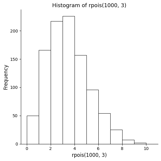
In the first command above, we generate a small sample of n=10 arrival delays, with a hoped for mean of 3 seconds of delay, just to see what kind of numbers we get. You can see that all of the numbers are small integers, ranging from 0 to 6. In the second command we double check these results with a slightly larger sample of n=100 to see if rpois() will hit the mean we asked for. In that run it came out to 2.99, which was pretty darned close. If you run this command yourself you will find that your result will vary a bit each time: it will sometimes be slightly larger than three and occasionally a little less than three (or whatever mean you specify). This is normal, because of the random number generator. In the third command we run yet another sample of 100 random data points, this time analyzing them with the var() function (which calculates the variance; see the chapter entitled “Beer, Farms, and Peas”). It is a curious fact of Poission distributions that the mean and the variance of the “ideal” (i.e., the theoretical) distribution are the same. In practice, for a small sample, they may be different.

In the final command, we ask for a histogram of an even larger sample of n=1000. The histogram shows the most common value hanging right around three seconds of delay with a nice tail that points rightwards and out to about 10 seconds of delay. You can think of this as one possible example of what you might observe of the average delay time between tweets was about three seconds. Note how similar the shape of this histogram is to what we observed with real tweets in the last chapter.

Compare the histogram on the previous page to the one on the next page that was generated with this command:

hist(rpois(1000,10))

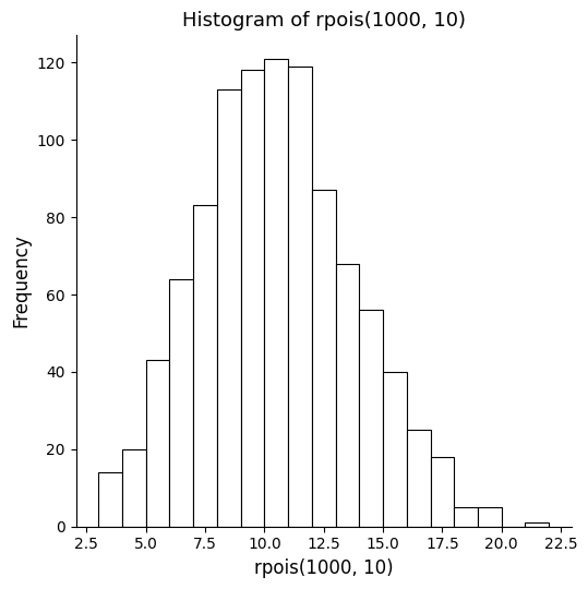
It is pretty easy to see the different shape and position of this histogram, which has a mean arrival delay of about ten seconds. First of all, there are not nearly as many zero length delays. Secondly, the most frequent value is now about 10 (as opposed to two in the previous histogram). Finally, the longest delay is now over 20 seconds (instead of 10 for the previous histogram). One other thing to try is this:

sum(rpois(1000,10)<=10)

[1] 597

This command generated 1000 new random numbers, following the Poisson distribution and also with a hoped-for mean of 10, just like in the histogram on the next page. Using the “<=” inequality test and the sum() function, we then counted up how many events were less than or equal to 12, and this turned out to be 597 events. As a fraction of the total of n=1000 data points that rpois() generated, that is 0.597, or 59.7%.