Introduction to Data Science Version 3

Yoiks, that last chapter was very challenging! Lots of numbers, lots of statistical concepts, lots of graphs. Let’s take a break from all that (temporarily) and focus on a different kind of data for a while. If you think about the Internet, and specifically about the World Wide Web for a while, you will realize: 1) That there are zillions of web pages; and 2) That most of the information on those web pages is “unstructured,” in the sense that it does not consist of nice rows and columns of numeric data with measurements of time or other attributes. Instead, most of the data spread out across the Internet is text, digital photographs, or digital videos. These last two categories are interesting, but we will have to postpone consideration of them while we consider the question of text.

Text is, of course, one of the most common forms of human communication, hence the label that researchers use sometimes: natural language. When we say natural language text we mean words created by humans and for humans. With our cool computer technology, we have collectively built lots of ways of dealing with natural language text. At the most basic level, we have a great system for representing individual characters of text inside of computers called “Unicode.” Among other things Unicode provides for a binary representation of characters in most of the world’s written languages, over 110,000 characters in all. Unicode supersedes ASCII (the American Standard Code for Information Interchange), which was one of the most popular standards (especially in the U.S.) for representing characters from the dawn of the computer age.

With the help of Unicode, most computer operating systems, and most application programs that handle text have a core strategy for representing text as lists of binary codes. Such lists are commonly referred to as “character strings” or in most cases just “strings.” One of the most striking things about strings from a computer programming perspective is that they seem to be changing their length all the time. You can’t perform the usual mathematical operations on character strings the way you can with numbers - no multiplication or division - but it is very common to “split” strings into smaller strings, and to “add” strings together to form longer strings. So while we may start out with, “the quick brown fox,” we may end up with “the quick brown” in one string and “fox” in another, or we may end up with something longer like, “the quick brown fox jumped over the lazy dog.”

Fortunately, R, like most other data handling applications, has a wide range of functions for manipulating, keeping track of, searching, and even analyzing string data. In this chapter, we will use our budding skills working with tweet data to learn the essentials of working with unstructured text data. The learning goal here is simply to become comfortable with examining and manipulating text data. We need these basic skills before we can tackle a more interesting problem.

Let’s begin by loading a new package, called “stringr”. Although R has quite a few string functions in its core, they tend to be a bit disorganized. So Hadley Wickham, a professor of statistics at Rice University, created this “stringr” package to make a set of string manipulation functions a bit easier to use and more comprehensive. You can install() and library() this package using the point and click features of R-Studio (look in the lower right hand pane under the Packages tab), or if you created the EnsurePackage() function from a couple of chapters back, you can use that:

EnsurePackage("stringr")

Now we can grab a new set of tweets with our custom function TweetFrame() from a couple of chapters ago (if you need the code, look in the chapter entitled “Tweet, Tweet”; we’ve also pasted the enhanced function, that sorts the tweets into arrival order, into the end of this chapter):

tweetDF <- TweetFrame("#solar",100)

This command should return a data frame containing about 100 tweets, mainly having to do with solar energy. You can choose any topic you like - all of the string techniques we examine in this chapter are widely applicable to any text strings. We should get oriented by taking a look at what we retrieved. The head() function can return the first entries in any vector or list:

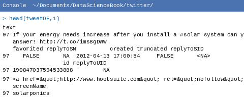
We provide a screen shot from R-Studio here just to preserve the formatting of this output. In the left hand margin, the number 97 represents R’s indexing of the original order in which the tweet was received. The tweets were re-sorted into arrival order by our enhanced TweetFrame() function (see the end of the chapter for code). So this is the first element in our dataframe, but internally R has numbered it as 97 out of the 100 tweets we obtained. On the first line of the output, R has place the label “text” and this is the field name of the column in the dataframe that contains the texts of the tweets. Other dataframe fields that we will not be using in this chapter include: “favorited,” “replyToSN,” and “truncated.” You may also recognize the field name “created” which contains the POSIX format time and date stamp that we used in previous chapters. Generally speaking, R has placed the example data (from tweet 97) that goes with the field name just underneath it, but the text justification can be confusing, and it makes this display very hard to read. For example, there is a really long number that starts with “1908” that is the unique numeric identifier (a kind of serial number) for this tweet. The field name “id” appears just above it, but is right justified (probably because the field is a number). The most important fact for us to note is that if we want to work with the text string that is the tweet itself, we need to use the field name “text.” Let’s see if we can get a somewhat better view if we use the head() function just on the text field. This command should provide just the first 2 entries in the “text” column of the dataframe:

head(tweetDF$text,2)

[1] "If your energy needs increase after you install a #solar system can you upgrade? Our experts have the answer! http://t.co/ims8gDWW"

[2] "#green New solar farms in West Tennessee signal growth: Two new solar energy farms producing electricity ... http://t.co/37PKAF3N #solar"

A couple of things which will probably seem obvious, but are nonetheless important to point out: The [1] and [2] are not part of the tweet, but are the typical line numbers that R uses in its output. The actual tweet text is between the double quotes. You can see the hashtag “#solar” appears in both tweets, which makes sense because this was our search term. There is also a second hashtag in the first tweet “#green” so we will have to be on the lookout for multiple hashtags. There is also a “shortened” URL in each of these tweets. If a Twitter user pastes in the URL of a website to which they want to refer people, the Twitter software automatically shortens the URL to something that begins with “http://t.co/” in order to save space in the tweet.

An even better way to look at these data, including the text and the other fields is to use the data browser that is built into R-Studio. If you look in the upper right hand pane of R-Studio, and make sure that the Workspace tab is clicked, you should see a list of available dataframes, under the heading “Data.” One of these should be “tweetDF.” If you click on tweetDF, the data browser will open in the upper left hand pane of R-Studio and you should be able to see the first field or two of the first dozen rows. 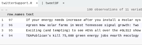Here’s a screen shot:

This screen shot confirms what we observed in the command line output, but gives us a much more appealing and convenient way of looking through our data. Before we start to manipulate our strings, let’s attach() tweetDF so that we don’t have to keep using the $ notation to access the text field. And before that, let’s check what is already attached with the search() function:

search()

[1] ".GlobalEnv"         "sortweetDF"         "package:gplots"
[4] "package:KernSmooth" "package:grid"       "package:caTools"

We’ve truncated this list to save space, but you can see on the first line “sortweetDF” left over from our work in a previous chapter. The other entries are all function packages that we want to keep active. So let’s detach() sortweetDF and attach tweetDF:

detach(sortweetDF)
attach(tweetDF)

These commands should yield no additional output. If you get any messages about “The following object(s) are masked from...” you should run search() again and look for other dataframes that should be detached before proceeding. Once you can run attach(“tweetDF”) without any warnings, you can be sure that the fields in this dataframe are ready to use without interference.