Introduction to Data Science Version 3

table(as.factor(rt))

The as.factor() function is a type/mode coercion and just a new one in a family we have seen before. In previous chapters we used as.integer() and as.character() to perform other conversions. In R a factor is a collection of descriptive labels and corresponding unique identifying numbers. The identifying numbers are not usually visible in outputs. Factors are often used for dividing up a dataset into categories. In a survey, for instance, if you had a variable containing the gender of a participant, the variable would frequently be in the form of a factor with (at least) two distinct categories (or what statisticians call levels), male and female. Inside R, each of these categories would be represented as a number, but the corresponding label would usually be the only thing you would see as output. As an experiment, try running this command:

str(as.factor(rt))

This will reveal the “structure” of the data object after coercion.

Returning to the earlier table(as.factor(rt)) command, the table() function takes as input one or more factors and returns a so called contingency table. This is easy to understand for use with just one factor: The function returns a unique list of factor “levels” (unique: meaning no duplicates) along with a count of how many rows/instances there were of each level in the dataset as a whole.

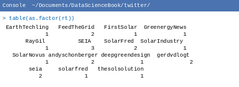
The screen shot on this page shows the command and the output. There are about 15 unique screennames of Twitter users who were retweeted. The highest number of times that a screenname appeared was three, in the case of SEIA. The table() function is used more commonly to create two-way (two dimensional) contingency tables. We could demonstrate that here if we had two factors, so let’s create another factor.

Remember earlier in the chapter we noticed some tweets had texts that were longer than 140 characters. We can make a new variable, we’ll call it longtext, that will be TRUE if the original tweet was longer than 140 characters and FALSE if it was not:

tweetDF$longtext <- (textlen>140)
detach(tweetDF)
attach(tweetDF)

The first command above has an inequality expression on the right hand side. This is tested for each row and the result, either TRUE or FALSE, is assigned to the new variable longtext. Computer scientists sometimes call this a “flag” variable because it flags whether or not a certain attribute is present in the data. Now we can run the table() function on the two factors:

table(as.factor(rt),as.factor(longtext))

FALSE TRUE
EarthTechling       0    1
FeedTheGrid         2    0
 FirstSolar          1    0
GreenergyNews       1    0
RayGil              0    1
SEIA                3    0
SolarFred           0    2
SolarIndustry       1    0
SolarNovus          1    0
andyschonberger     0    2
deepgreendesign     0    1
gerdvdlogt          2    0
seia                2    0
solarfred           1    0
thesolsolution      1    0

For a two-way contingency table, the first argument you supply to table() is used to build up the rows and the second argument is used to create the columns. The command and output above give us a nice compact display of which retweets are longer than 140 characters (the TRUE column) and which are not (the FALSE column). It is easy to see at a glance that there are many in each category. So, while doing a retweet may contribute to having an extra long tweet, there are also many retweets that are 140 characters or less. It seems a little cumbersome to look at the long list of retweet screennames, so we will create another flag variable that indicates whether a tweet text contains a retweet. This will just provide a more compact way of reviewing which tweets have retweets and which do not:

tweetDF$hasrt <- !(is.na(rt))
detach(tweetDF)
attach(tweetDF)
View(tweetDF)

The first command above uses a function we have not encountered bevfore: is.na(). A whole family of functions that start with “is” exists in R (as well as in other programming languages) and these functions provide a convenient way of testing the status or contents of a data object or of a particular element of a data object. The is.na() function tests whether an element of the input variable has the value NA, which we know from earlier in the chapter is R’s way of showing a missing value (when a particular data element is empty). So the expression, is.na(rt) will return TRUE if a particular cell of tweetDF$rt contains the empty value NA, and false if it contains some real data. If you look at the name of our new variable, however, which we have called “hasrt” you may see that we want to reverse the sense of the TRUE and FALSE that is.na() returns. To do that job we use the “!” character, which computers scientists may either call “bang” or more accurately, “not.” Using “not” is more accurate because the “!” character provides the Boolean NOT function, which changes a TRUE to a FALSE and vice versa. One last little thing is that the View() command causes R-Studio to freshen the display of the dataframe in its upper left hand pane. Let’s look again at retweets and long tweet texts:

table(hasrt,longtext)

longtext
hasrt   FALSE TRUE
FALSE    76    2
TRUE     15    7

There are more than twice as many extra long texts (7) when a tweet contains a retweet than when it does not.

Let’s now follow the same general procedure for extracting the URLs from the tweet texts. As before the goal is to create a new string variable/column on the original dataframe that will contain the URLs for all of those tweets that have them. Additionally, we will create a flag variable that signifies whether or not each tweet contains a URL. Here, as before, we follow a key principle: Don’t mess with your original data. We will need to develop a new regular expression in order to locate an extract the URL string from inside of the tweet text. Actually, if you examine your tweet data in the R-Studio data browser, you may note that some of the tweets have more than one URL in them. So we will have to choose our function call carefully and be equally careful looking at the results to make sure that we have obtained what we need.

At the time when this was written, Twitter had imposed an excellent degree of consistency on URLs, such that they all seem to start with the string “http://t.co/”. Additionally, it seems that the compacted URLs all contain exactly 8 characters after that literal, composed of upper and lower case letters and digits. We can use str_match_all() to extract these URLs using the following code:

str_match_all(text,"http://t.co/[a-z,A-Z,0-9]{8}")

We feed the tweetDF$text field as input into this function call (we don’t need to provide the tweetDF$ part because this dataframe is attached). The regular expression begins with the 12 literal characters ending with a forward slash. Then we have a regular expression pattern to match. The material within the square brackets matches any upper or lowercase letter and any digit. The numeral 8 between the curly braces at the end say to match the previous pattern exactly eight times. This yields output that looks like this:

[[6]]
     [,1]
[1,] "http://t.co/w74X9jci"

[[7]]
     [,1]
[1,] "http://t.co/DZBUoz5L"
[2,] "http://t.co/gmtEdcQI"

This is just an excerpt of the output, but there are a couple of important things to note. First, note that the first element is preceded by the notation [[6]]. In the past when R has listed out multiple items on the output, we have seen them with index numbers like [1] and [2]. In this case, however, that could be confusing because each element in the output could have multiple rows (as item [[7]] above clearly shows). So R is using double bracket notation to indicate the ordinal number of each chunk of data in the list, where a given chunk may itself contain multiple elements.

Confusing? Let’s go at it from a different angle. Look at the output under the [[7]] above. As we noted a few paragraphs ago, some of those tweets have multiple URLs in them. The str_match_all() function handles this by creating, for every single row in the tweet data, a data object that itself contains exactly one column but one or possibly more than one row - one row for each URL that appears in the tweet. So, just as we saw earlier in the chapter, we are getting back from a string function a complex matrix-like data object that requires careful handling if we are to make proper use of it.

The only other bit of complexity is this: What if a tweet contained no URLs at all? Your output from running the str_match_all() function probably contains a few elements that look like this:

[[30]]
character(0)

[[31]]
character(0)

So elements [[30]] and [[31]] of the data returned from str_match_all() each contain a zero length string. No rows, no columns, just character(0), the so-called null character, which in many computer programming languages is used to “terminate” a string.

Let’s go ahead and store the output from str_match_all() into a new vector on tweetDF and then see what we can do to tally up the URLs we have found:

tweetDF$urlist<-str_match_all(text,+
                 "http://t.co/[a-z,A-Z,0-9]{8}")
detach(tweetDF)
attach(tweetDF)
head(tweetDF$urlist,2)

[[1]]
     [,1]
[1,] "http://t.co/ims8gDWW"

[[2]]
     [,1]
[1,] "http://t.co/37PKAF3N"

Now we are ready to wrestle with the problem of how to tally up the results of our URL parsing. Unlike the situation with retweets, where there either was or was not a single retweet indication in the text, we have the possibility of zero, one or more URLs within the text of each tweet. Our new object “urlist” is a multi-dimensional object that contains a single null character, one row/column of character data, or one column with more than one row of character data. The key to summarizing this is the length() function, which will happily count up the number of elements in an object that you supply to it:

length(urlist[[1]])

[1] 1

length(urlist[[5]])

[1] 0

length(urlist[[7]])

[1] 2

Here you see that double bracket notation again, used as an index into each “chunk” of data, where the chunk itself may have some internal complexity. In the case of element [[1]] above, there is one row, and therefore one URL. For element [[5]] above, we see a zero, which means that length() is telling us that this element has no rows in it at all. Finally, for element [[7]] we see 2, meaning that this element contains two rows, and therefore two URLs.

In previous work with R, we’ve gotten used to leaving the inside of the square brackets empty when we want to work with a whole list of items, but that won’t work with the double brackets:

length(urlist[[]])

Error in urlist[[]] : invalid subscript type 'symbol'

The double brackets notation is designed to reference just a single element or component in a list, so empty double brackets does not work as a shorthand for every element in a list. So what we must do if we want to apply the length() function to each element in urlist is to loop. We could accomplish this with a for loop, as we did in the last chapter, using an index quantity such as “i” and substituting i into each expression like this: urlist[[i]]. But let’s take this opportunity to learn a new function in R, one that is generally more efficient for looping. The rapply() function is part of the “apply” family of functions, and it stands for “recursive apply.” Recursive in this case means that the function will dive down into the complex, nested structure of urlist and repetitively run a function for us, in this case the length() function:

tweetDF$numurls<-rapply(urlist,length)
detach(tweetDF)
attach(tweetDF)
head(numurls,10)

[1] 1 1 1 1 0 1 2 1 1 1

Excellent! We now have a new field on tweetDF that counts up the number of URLs. As a last step in examining our tweet data, let’s look at a contingency table that looks at the number of URLs together with the flag indicating an extra long tweet. Earlier in the chapter, we mentioned that the table() function takes factors as its input. In the command below we have supplied the numurls field to the table() function without coercing it to a factor. Fortunately, the table() function has some built in intelligence that will coerce a numeric variable into a factor. In this case because numurls only takes on the values of 0, 1, or 2, it makes good sense to allow table() to perform this coercion:

table(numurls,longtext)

longtext

numurls FALSE TRUE
0    16    3
1    72    6
2     3    0

This table might be even more informative if we looked at it as proportions, so here is a trick to view proportions instead of counts:

prop.table(table(numurls,longtext))

longtext

numurls FALSE TRUE
0  0.16 0.03
1  0.72 0.06
2  0.03 0.00

That looks familiar! Now, of course, we remember that we had exactly 100 tweets, so each of the counts could be considered a percentage with no further calculation. Still, prop.table() is a useful function to have when you would rather view your contingency tables as percentages rather than counts. We can see from these results that six percent of the tweets have one URL, but only three percent have no URLS.

So, before we close out this chapter, let’s look at a three way contingency table by putting together our two flag variables and the number of URLs:

table(numurls,hasrt,longtext)

, , longtext = FALSE
hasrt

numurls FALSE TRUE
0    15    1
1    58   14
2     3    0

, , longtext = TRUE
hasrt
numurls FALSE TRUE
0     0    3
1     2    4
2     0    0

Not sure this entirely solves the mystery, but if we look at the second two-way table above, where longtext = TRUE, it seems that extra long tweets either have a retweet (3 cases), or a single URL (2 cases) or both (4 cases).

When we said we would give statistics a little rest in this chapter, we lied just a tiny bit. Check out these results:

mean(textlen[hasrt&longtext])

[1] 155

mean(textlen[!hasrt&longtext])

[1] 142

In both commands we have requested the mean of the variable textlen, which contains the length of the original tweet (the one without the space stripped out). In each command we have also used the bracket notation to choose a particular subset of the cases. Inside the brackets we have a logical expression. The only cases that will be included in the calculation of the mean are those where the expression inside the brackets evaluates to TRUE. In the first command we ask for the mean tweet length for those tweets that have a retweet AND are extra long (the ampersand is the Boolean AND operator). In the second command we use the logical NOT (the “!” character) to look at only those cases that have extra long text but do not have a retweet. The results are instructive. The really long tweets, with a mean length of 155 characters, are those that have retweets. It seems that Twitter does not penalize an individual who retweets by counting the number of characters in the “RT @SCREENNAME:” string. If you have tried the web interface for Twitter you will see why this makes sense: Retweeting is accomplished with a click, and the original tweet - which after all may already be 140 characters - appears underneath the screenname of the originator of the tweet. The “RT @” string does not even appear in the text of the tweet at that point.

Looking back over this chapter, we took a close look at some of the string manipulation functions provided by the package “stringr”. These included some of the most commonly used actions such as finding the length of a string, finding matching text within a string, and doing search and replace operations on a string. We also became aware of some additional complexity in nested data structures. Although statisticians like to work with nice, well-ordered rectangular datasets, computer scientists often deal with much more complex data structures - although these are built up out of parts that we are familiar with such as lists, vectors, and matrices.

Twitter is an excellent source of string data, and although we have not yet done much in analyzing the contents of tweets or their meanings, we have looked at some of the basic features and regularities of the text portion of a tweet. In the next chapter we will become familiar with a few additional text tools and then be in a position to manipulate and analyze text data