Section 16.2 Geocoding and Combining Data
Next, we need a source of points to add to our map. This could be anything that we’re interested in: the locations of restaurants, crime scenes, colleges, etc. In Google a search for filetype:xls or filetype;csv with appropriate additional search terms can provide interesting data sources. You may also have mailing lists of customers or clients. The most important thing is that we will need street address, city, and state in order to geocode the addresses. For this example, we searched for “housing street address list filetype:csv” and this turned up a data set of small businesses that have contracts with the U.S. Department of Health and Human services. Let’s read this in using read.csv():
dhhsAddrs <- read.csv("DHHS_Contracts.csv")
str(dhhsAddrs)
'data.frame':	599 obs. of  10 variables:
$ Contract.Number           : Factor w/ 285 levels "26301D0054","500000049",..: 125 125 125 279 164 247 19 242 275 70 ...
$ Contractor.Name           : Factor w/ 245 levels "2020 COMPANY LIMITED LIABILITY COMPANY",..: 1 1 1 2 2 3 4 6 5 7 ...
$ Contractor.Address        : Factor w/ 244 levels "1 CHASE SQUARE 10TH FLR, ROCHESTER, NY ",..: 116 116 116 117 117 136 230 194 64 164 ...
$ Description.Of.Requirement: Factor w/ 468 levels "9TH SOW - DEFINTIZE THE LETTER CONTRACT",..: 55 55 55 292 172 354 308 157 221 340 ...
$ Dollars.Obligated         : Factor w/ 586 levels " $1,000,000.00 ",..: 342 561 335 314 294 2 250 275 421 21 ...
$ NAICS.Code                : Factor w/ 55 levels "323119","334310",..: 26 26 26 25 10 38 33 29 27 35 ...
$ Ultimate.Completion.Date  : Factor w/ 206 levels "1-Aug-2011","1-Feb-2013",..: 149 149 149 10 175 161 124 37 150 91 ...
$ Contract.Specialist       : Factor w/ 95 levels "ALAN  FREDERICKS",..: 14 14 60 54 16 90 55 25 58 57 ...
$ Contract.Specialist.Email : Factor w/ 102 levels "410-786-8622",..: 16 16 64 59 40 98 60 29 62 62 ...
$ X               : logi  NA NA NA NA NA NA ...
There’s that crazy 60s song again! Anyhow, we read in a comma separated data set with 599 rows and 10 variables. The most important field we have there is Contractor.Address. This contains the street addresses that we need to geocode. We note, however, that the data type for these is Factor rather than character string. So we need to convert that:
dhhsAddrs$strAddr <- +
       as.character(dhhsAddrs$Contractor.Address)
mode(dhhsAddrs$strAddr)
[1] "character"
tail(dhhsAddrs$strAddr,4)
[1] "1717 W BROADWAY, MADISON, WI "
[2] "1717 W BROADWAY, MADISON, WI "
[3] "1717 W BROADWAY, MADISON, WI "
[4] "789 HOWARD AVE, NEW HAVEN, CT, "
This looks pretty good: Our new column, called dhhsAddrs, is character string data, converted from the factor labels of the original Contractor.Address column. Now we need to geocode these. We will use the Google geocoding application programming interface (API) which is pretty easy to use, does not require an account or application ID, and allows about 2500 address conversions per day. The API can be accessed over the web, using what is called an HTTP GET request. Note that the Terms of Service for the Google geocoding API are very specific about how the interface can be used - most notably on the point that the geocodes must be used on Google maps. Make sure you read the Terms of Service before you create any software applications that use the geocoding service. See the link in the bibliography at the end of the chapter. The bibliography has a link to an article with dozens of other geocoding APIs if you disagree with Google’s Terms of Service.
These acronyms probably look familiar. HTTP is the Hyper Text Transfer Protocol, and it is the standard method for requesting and receiving web page data. A GET request consists of information that is included in the URL string to specify some details about the information we are hoping to get back from the request. Here is an example GET request to the Google geocoding API:
The first part of this should look familiar: The http://maps.googleapis.com part of the URL specifies the domain name just like a regular web page. The next part of the URL,
“/maps/api/geocode” tells Google which API we want to use. Then the “json” indicates that we would like to receive our result in “Java Script Object Notation” (JSON) which is a structured, but human readable way of sending back some data. The address appears next, and we are apparently looking for the White House at 1600 Pennsylvania Avenue in Washington, DC. Finally, sensor=false is a required parameter indicating that we are not sending our request from a mobile phone. You can type that whole URL into the address field of any web browser and you should get a sensible result back. The JSON notation is not beautiful, but you will see that it makes sense and provides the names of individual data items along with their values. Here’s a small excerpt that shows the key parts of the data object that we are trying to get our hands on:
{
"results" : [
    {
        "address_components" : [
        "geometry" : {
            "location" : {
                "lat" : 38.89788009999999,
                "lng" : -77.03664780
            },
   "status" : "OK"
  }
There’s tons more data in the JSON object that Google returned, and fortunately there is an R package, called JSONIO, that will extract the data we need from the structure without having to parse it ourselves.
In order to get R to send the HTTP GET requests to google, we will also need to use the RCurl package. This will give us a single command to send the request and receive the result back - essentially doing all of the quirky steps that a web browser takes care of automatically for us. To get started, install.packages() and library() the two packages we will need - RCurl and JSONIO. If you are working on a Windows machine, you may need to jump through a hoop or two to get RCurl, but it is available for Windows even if it is not in the standard CRAN repository. Search for “RCurl Windows” if you run into trouble.
Next, we will create a new helper function to take the address field and turn it into the URL that we need:
# Format an URL for the Google Geocode API
MakeGeoURL <- function(address)
{
root <- "http://maps.google.com/maps/api/geocode/"
url <- paste(root, "json?address=",    address, "&sensor=false", sep = "")
return(URLencode(url))
}
There are three simple steps here. The first line initializes the beginning part of the URL into a string called root. Then we use
paste() to glue together the separate parts of the strong (note the sep=”” so we don’t get spaces between the parts). This creates a string that looks almost like the one in the White House example two pages ago. The final step converts the string to a legal URL using a utility function called URLencode() that RCurl provides. Let’s try it:
MakeGeoURL("1600 Pennsylvania Avenue, Washington, DC")
[1] "http://maps.google.com/maps/api/geocode/json?address=1600%20Pennsylvania%20Avenue,%20Washington,%20DC&sensor=false"
Looks good! Just slightly different than the original example (%20 instead of the plus character) but hopefully that won’t make a difference. Remember that you can type this function at the command line or you can create it in the script editing window in the upper left hand pane of R-Studio. The latter is the better way to go and if you click the “Source on Save” checkmark, R-Studio will make sure to update R’s stored version of your function every time you save the script file.
Now we are ready to use our new function,
MakeGeoURL(), in another function that will actually request the data from the Google API:
Addr2latlng <- function(address)
{
url <- MakeGeoURL(address)
apiResult <- getURL(url)
geoStruct <- fromJSON(apiResult, +
                               simplify = FALSE)
lat <- NA
lng <- NA
try(lat <- +
    geoStruct$results[[1]]$geometry$location$lat)
try(lng <- +
    geoStruct$results[[1]]$geometry$location$lng)
return(c(lat, lng))
}
We have defined this function to receive an address string as its only argument. The first thing it does is to pass the URL string to
MakeGeoURL() to develop the formatted URL. Then the function passes the URL to getURL(), which actually does the work of sending the request out onto the Internet. The getURL() function is part of the RCurl package. This step is just like typing a URL into the address box of your browser.
We capture the result in an object called “apiResult”. If we were to stop and look inside this, we would find the JSON structure that appeared a couple of pages ago. We can pass this structure to the function
fromJSON() - we put the result in an object called geoStruct. This is a regular R data frame such that we can access any individual element using regular $ notation and the array index [[1]]. In other instances, a JSON object may contain a whole list of data structures, but in this case there is just one. If you compare the variable names “geometry”, “location”, “lat” and “lng” to the JSON example a few pages ago you will find that they match perfectly. The fromJSON() function in the JSONIO package has done all the heavy lifting of breaking the JSON structure into its component pieces.
Note that this is the first time we have encountered the try() function. When programmers expect the possibility of an error, they will frequently use methods that are tolerant of errors or that catch errors before they disrupt the code. If our call to getURL() returns something unusual that we aren’t expecting, then the JSON structure may not contain the fields that we want. By surrounding our command to assign the lat and lng variables with a try() function, we can avoid stopping the flow of the code if there is an error. Because we initialized lat and lng to NA above, this function will return a two item list with both items being NA if an error occurs in accessing the JSON structure. There are more elegant ways to accomplish this same goal. For example, the Google API puts an error code in the JSON structure and we could choose to interpret that instead. We will leave that to the chapter challenge!
In the last step, our new
Addr2latlng() function returns a two item list containing the latitude and longitude. We can test it out right now:
testData <- Addr2latlng( +
      "1600 Pennsylvania Avenue, Washington, DC")
str(testData)
num [1:2] 38.9 -77
Perfect! we called our new function
Addr2latlng() with the address of the White House and got back a list with two numeric items containing the latitude and longitude associate with that address. With just a few lines of R code we have harnessed the power of Google’s extensive geocoding capability to convert a brief text street address into mapping coordinates.
At this point there isn’t too much left to do. We have to create a looping mechanism so that we can process the whole list of addresses in our DHHS data set. We have some small design choices here. It would be possible to attach new fields to the existing dataframe. Instead, the following code keeps everything pretty simple by receiving a list of addresses and returning a new data frame with X, Y, and EID ready to feed into our mapping software:
# Process a whole list of addresses
ProcessAddrList <- function(addrList)
{
resultDF <- data.frame(atext=character(),    X=numeric(),Y=numeric(),EID=numeric())
i <- 1
for (addr in addrList)
{
latlng = Addr2latlng(addr)
resultDF <- rbind(resultDF,      data.frame(atext=addr,       X=latlng[[2]],Y=latlng[[1]], EID=i))
i <- i + 1
}
return(resultDF)
}
This new function takes one argument, the list of addresses, which should be character strings. In the first step we make an empty dataframe for use in the loop. In the second step we initialize a scalar variable called i to the number one. We will increment this in the loop and use it as our EID.
Then we have the for loop. We are using a neat construct here called “in”. The expression “addr in addrList” creates a new variable called addr. Every time that R goes through the loop it assigns to addr the next item in addrList. When addrList runs out of items, the for loop ends. Very handy!
Inside the for loop the first thing we do is to call the function that we developed earlier:
Addr2latlng(). This performs one conversion of an address to a geocode (latitude and longitude) as described earlier. We pass addr to it as add contains the text address for this time around the loop. We put the result in a new variable called latlng. Remember that this is a two item list.
The next statement, starting with “resultDF <- rbind” is the heart of this function. Recall that
rbind() sticks a new row on the end of a dataframe. So in the arguments to rbind() we supply our earlier version of resultDF (which starts empty and grows from there) plus a new row of data. The new row of data includes the text address (not strictly necessary but handy for diagnostic purposes), the “X” that our mapping software expects (this is the longitude), the “Y” that the mapping software expects, and the event ID, EID, that the mapping software expects.
At the end of the for loop, we increment i so that we will have the next number next time around for EID. Once the for loop is done we simply return the dataframe object, resultDF. Piece of cake!
Now let’s try it and plot our points:
dhhsPoints <- ProcessAddrList(dhhsAddrs$strAddr)
dhhsPoints <- dhhsPoints[!is.na(dhhsPoints$X),]
eventData <- as.EventData(dhhsPoints,projection=NA)
addPoints(eventData,col="red",cex=.5)
The second command above is the only one of the four that may seem unfamiliar. The
as.EventData() coercion is picky and will not process the dataframe if there are any fields that are NA. To get rid of those rows that do not have complete latitude and longitude data, we use is.na() to test whether the X value on a given row is NA. We use the ! (not) operator to reverse the sense of this test. So the only rows that will survive this step are those where X is not NA. The plot below shows the results.
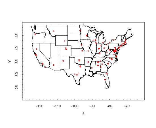
If you like conspiracy theories, there is some support in this graph: The vast majority of the companies that have contracts with DHHS are in the Washington, DC area, with a little trickle of additional companies heading up the eastern seaboard as far as Boston and southern New Hampshire. Elsewhere in the country there are a few companies here and there, particularly near the large cities of the east and south east.
Using some of the parameters on
plotPolys() you could adjust the zoom level and look at different parts of the country in more detail. If you remember that the original DHHS data also had the monetary size of the contract in it, it would also be interesting to change the size or color of the dots depending on the amount of money in the Dollars.Obligated field. This would require running addPoints() in a loop and setting the col= or cex= parameters for each new point.

