Introduction to Data Science Version 3

Conveniently, R has a function called sample(), that will draw a random sample from a data set with just a single call. We can try it now with our state data:

sample(USstatePops$V1,size=16,replace=TRUE)

[1] 4533372 19378102 897934 1052567 672591
18801310 2967297
[8] 5029196

As a matter of practice, note that we called the sample() function with three arguments. The first argument was the data source. For the second and third arguments, rather than rely on the order in which we specify the arguments, we have used “named arguments” to make sure that R does what we wanted. The size=16 argument asks R to draw a sample of 16 state data values. The replace=TRUE argument specifies a style of sampling which statisticians use very often to simplify the mathematics of their proofs. For us, sampling with or without replacement does not usually have any practical effects, so we will just go with what the statisticians typically do.

When we’re working with numbers such as these state values, instead of counting gumball colors, we’re more interested in finding out the average, or what you now know as the mean. So we could also ask R to calculate a mean() of the sample for us:

mean(sample(USstatePops$V1,size=16,
replace=TRUE))

[1] 8198359

There’s the nested function call again. The output no longer shows the eight values that R sampled from the list of 51. Instead it used those eight values to calculate the mean and display that for us. If you have a good memory, or merely took the time to look in the last chapter, you will remember that the actual mean of our 51 observations is 6,053,834. So the mean that we got from this one sample of eight states is really not even close to the true mean value of our 51 observations. Are we worried? Definitely not! We know that when we draw a sample, whether it is gumballs or states, we will never hit the true population mean right on the head. We’re interested not in any one sample, but in what happens over the long haul. So now we’ve got to get R to repeat this process for us, not once, not four times, but four hundred times or four thousand times. Like most programming languages, R has a variety of ways of repeating an activity. One of the easiest ones to use is the replicate() function. To start, let’s just try four replications:

replicate(4, mean(sample(USstatePops$V1, size=16,replace=TRUE)),simplify=TRUE)

[1] 10300486 11909337 8536523 5798488

Couldn’t be any easier. We took the exact same command as before, which was a nested function to calculate the mean() of a random sample of eight states (shown above in bold). This time, we put that command inside the replicate() function so we could run it over and over again. The simplify=TRUE argument asks R to return the results as a simple vector of means, perfect for what we are trying to do. We only ran it four times, so that we would not have a big screen full of numbers. From here, though, it is easy to ramp up to repeating the process four hundred times. You can try that and see the output, but for here in the book we will encapsulate the whole replicate function inside another mean(), so that we can get the average of all 400 of the sample means. Here we go:

mean(replicate(400, mean(
sample(USstatePops$V1,size=16,replace=TRUE)),
simplify=TRUE))

[1] 5958336

In the command above, the outermost mean() command is bolded to show what is different from the previous command. So, put into words, this deeply nested command accomplishes the following: a) Draw 400 samples of size n=8 from our full data set of 51 states; b) Calculate the mean from each sample and keep it in a list; c) When finished with the list of 400 of these means, calculate the mean of that list of means. You can see that the mean of four hundred sample means is 5,958,336. Now that is still not the exact value of the whole data set, but it is getting close. We’re off by about 95,000, which is roughly an error of about 1.6% (more precisely, 95,498/6,053,834 = 1.58%. You may have also noticed that it took a little while to run that command, even if you have a fast computer. There’s a lot of work going on there! Let’s push it a bit further and see if we can get closer to the true mean for all of our data:

mean(replicate(4000, mean(
sample(USstatePops$V1,size=16,replace=TRUE)),
simplify=TRUE))

[1] 6000972

Now we are even closer! We are now less than 1% away from the true population mean value. Note that the results you get may be a bit different, because when you run the commands, each of the 400 or 4000 samples that is drawn will be slightly different than the ones that were drawn for the commands above. What will not be much different is the overall level of accuracy.

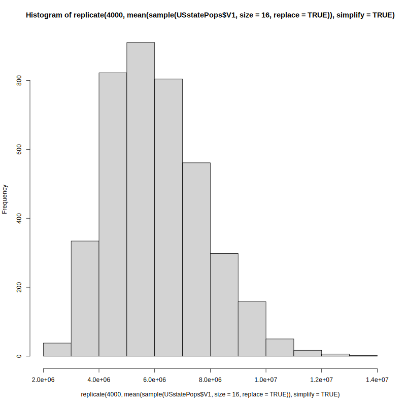
We’re ready to take the next step. Instead of summarizing our whole sampling distribution in a single average, let’s look at the distribution of means using a histogram.

The histogram displays the complete list of 4000 means as frequencies. Take a close look so that you can get more practice reading frequency histograms. This one shows a very typical configuration that is almost bell-shaped, but still has a bit of “skewness” off to the right. The tallest, and therefore most frequent range of values is right near the true mean of 6,053,834.

By the way, were you able to figure out the command to generate this histogram on your own? All you had to do was substitute hist() for the outermost mean() in the previous command. In case you struggled, here it is:

hist(replicate(4000, mean(
sample(USstatePops$V1,size=16,replace=TRUE)),
simplify=TRUE))

This is a great moment to take a deep breath. We’ve just covered a couple hundred years of statistical thinking in just a few pages. In fact, there are two big ideas, “the law of large numbers” and the central limit theorem” that we have just partially demonstrated. These two ideas literally took mathematicians like Gerolamo Cardano (1501-1576) and Jacob Bernoulli (1654-1705) several centuries to figure out. If you look these ideas up, you may find a lot of bewildering mathematical details, but for our purposes, there are two really important take-away messages. First, if you run a statistical process a large number of times, it will converge on a stable result. For us, we knew what the average population was of the 50 states plus the District of Columbia. These 51 observations were our population, and we wanted to know how many smaller subsets, or samples, of size n=16 we would have to draw before we could get a good approximation of that true value. We learned that drawing one sample provided a poor result. Drawing 400 samples gave us a mean that was off by 1.5%. Drawing 4000 samples gave us a mean that was off by less than 1%. If we had kept going to 40,000 or 400,000 repetitions of our sampling process, we would have come extremely close to the actual average of 6,053,384.

Second, when we are looking at sample means, and we take the law of large numbers into account, we find that the distribution of sampling means starts to create a bell-shaped or normal distribution, and the center of that distribution, the mean of all of those sample means gets really close to the actual population mean. It gets closer faster for larger samples, and in contrast, for smaller samples you have to draw lots and lots of them to get really close. Just for fun, lets illustrate this with a sample size that is larger than 16. Here’s a run that only repeats 100 times, but each time draws a sample of n=51 (equal in size to the population):

mean(replicate(100, mean(
sample(USstatePops$V1,size=51,replace=TRUE)),
simplify=TRUE))

[1] 6114231

Now, we’re only off from the true value of the population mean by about one tenth of one percent. You might be scratching your head now, saying, “Wait a minute, isn’t a sample of 51 the same thing as the whole list of 51 observations?” This is confusing, but it goes back to the question of sampling with replacement that we examined a couple of pages ago (and that appears in the command above as replace=TRUE). Sampling with replacement means that as you draw out one value to include in your random sample, you immediately chuck it back into the list so that, potentially, it could get drawn again either immediately or later. As mentioned before, this practice simplifies the underlying proofs, and it does not cause any practical problems, other than head scratching. In fact, we could go even higher in our sample size with no trouble:

mean(replicate(100, mean(
sample(USstatePops$V1,size=120,replace=TRUE)),
simplify=TRUE))

[1] 6054718

That command runs 100 replications using samples of size n=120. Look how close the mean of the sampling distribution is to the population mean now! Remember that this result will change a little bit every time you run the procedure, because different random samples are being drawn for each run. But the rule of thumb is that the bigger your sample size, what statisticians call n, the closer your estimate will be to the true value. Likewise, the more trials you run, the closer your population estimate will be.