Introduction to Data Science Version 3

As a first step we need to install and library() the “wordcloud” package. As with other packages, either use the package interface in R-Studio or the EnsurePackage() function that we wrote a few chapters ago. The wordcloud package was written by freelance statistician Ian Fellows, who also developed the “Deducer” user interface for R. Deducer provides a graphical interface that allows users who are more familiar with SPSS or SAS menu systems to be able to use R without resorting to the command line.

Once the wordcloud package is loaded, we need to do a little preparation to get our data ready to submit to the word cloud generator function. That function expects two vectors as input arguments, the first a list of the terms, and the second a list of the frequencies of occurrence of the terms. The list of terms and frequencies must be sorted with the most frequent terms appearing first. To accomplish this we first have to coerce our tweet data back into a plain data matrix so that we can sort it by frequency. The first command below accomplishes this:

tdMatrix <- as.matrix(tweetTDM)
sortedMatrix<-sort(rowSums(tdMatrix),+
                              decreasing=TRUE)
cloudFrame<-data.frame( +
   word=names(sortedMatrix),freq=sortedMatrix)
wordcloud(cloudFrame$word,cloudFrame$freq)

In the next command above, we are accomplishing two things in one command: We are calculating the sums across each row, which gives us the total frequency of a term across all of the different tweets/documents. We are also sorting the resulting values with the highest frequencies first. The result is a named list: Each item of the list has a frequency and the name of each item is the term to which that frequency applies.

In the second to last command above, we are extracting the names from the named list in the previous command and binding them together into a dataframe with the frequencies. This dataframe, “cloudFrame”, contains exactly the same information as the named list. “sortedMatrix,” but cloudFrame has the names in a separate column of data. This makes it easier to do the final command above, which is the call to the wordcloud() function. The wordcloud() function has lots of optional parameters for making the word cloud more colorful, controlling its shape, and controlling how frequent an item must be before it appears in the cloud, but we have used the default settings for all of these parameters for the sake of simplicity. We pass to the wordcloud() function the term list and frequency list that we bound into the dataframe and wordcloud() produces the nice graphic that you see below.

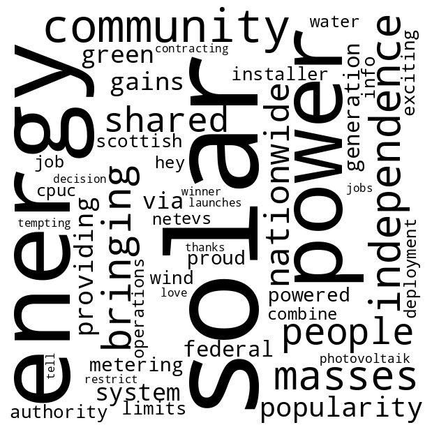
If you recall the Twitter search that we used to retrieve those tweets (#solar) it makes perfect sense that “solar” is the most frequent term (even though we filtered out all of the hashtags. The next most popular term is “energy” and after that there are a variety of related words such as “independence,” “green,” “wind,” and “metering.”