Section 10.2 Writing Your First Function
The upper left hand “pane” (another name for a sub-window) displays a blank space under the tab title “Untitled1.” Click in that pane and type the following:
MyMode <- function(myVector)
{
return(myVector)
}
You have just created your first “function” in R. A function is a bundle of R code that can be used over and over again without having to retype it. Other programming languages also have functions. Other words for function are “procedure” and “subroutine,” although these terms can have a slightly different meaning in other languages. We have called our function
MyMode(). You may remember from a couple of chapters that the basic setup of R does not have a statistical mode function in it, even though it does have functions for the two other other common central tendency statistics, mean() and median(). We’re going to fix that problem by creating our own mode function. Recall that the mode function should count up how many of each value is in a list and then return the value that occurs most frequently. That is the definition of the statistical mode: the most frequently occurring item in a vector of numbers.
A couple of other things to note: The first is the “myVector” in parentheses on the first line of our function. This is the “argument” or input to the function. We have seen arguments before when we called functions like
mean() and median(). Next, note the curly braces that are used on the second and final lines. These curly braces hold together all of the code that goes in our function. Finally, look at the return() right near the end of our function. This return() is where we send back the result of what our function accomplished. Later on when we “call” our new function from the R console, the result that we get back will be whatever is in the parentheses in the return().
Based on that explanation, can you figure out what
MyMode() does in this primitive initial form? All it does is return whatever we give it in myVector, completely unchanged. By the way, this is a common way to write code, by building up bit by bit. We can test out what we have each step of the way. Let’s test out what we have accomplished so far. First, let’s make a very small vector of data to work with. In the lower left hand pane of R-studio you will notice that we have a regular R console running. You can type commands into this console, just like we did in previous chapters just using R:
tinyData <- c(1,2,1,2,3,3,3,4,5,4,5)
tinyData
[1] 1 2 1 2 3 3 3 4 5 4 5
Then we can try out our new
MyMode() function:
MyMode(tinyData)
Error: could not find function "MyMode"
Oops! R doesn’t know about our new function yet. We typed our
MyMode() function into the code window, but we didn’t tell R about it. If you look in the upper left pane, you will see the code for MyMode() and just above that a few small buttons on a tool bar. One of the buttons looks like a little right pointing arrow with the word “Run” next to it. First, use your mouse to select all of the code for MyMode(), from the first M all the way to the last curly brace. Then click the Run button. You will immediately see the same code appear in the R console window just below. If you have typed everything correctly, there should be no errors or warnings. Now R knows about our MyMode() function and is ready to use it. Now we can type:
MyMode(tinyData)
[1] 1 2 1 2 3 3 3 4 5 4 5
This did exactly what we expected: it just echoed back the contents of
tinyData. You can see from this example how parameters work, too. In the command just above, we passed in tinyData as the input to the function. While the function was working, it took what was in tinyData and copied it into myVector for use inside the function. Now we are ready to add the next command to our function:
MyMode <- function(myVector)
{
uniqueValues <- unique(myVector)
return(uniqueValues)
}
Because we made a few changes, the whole function appears again above. Later, when the code gets a little more complicated, we will just provide one or two lines to add. Let’s see what this code does. First, don’t forget to select the code and click on the Run button. Then, in the R console, try the
MyMode() command again:
MyMode(tinyData)
[1] 1 2 3 4 5
Pretty easy to see what the new code does, right? We called the
unique() function, and that returned a list of unique values that appeared in tinyData. Basically, unique() took out all of the redundancies in the vector that we passed to it. Now let’s build a little more:
MyMode <- function(myVector)
{
uniqueValues <- unique(myVector)
uniqueCounts <- tabulate(myVector)
return(uniqueCounts)
}
Don’t forget to select all of this code and Run it before testing it out. This time when we pass tinyData to our function we get back another list of five elements, but this time it is the count of how many times each value occurred:
MyMode(tinyData)
[1] 2 2 3 2 2
Now we’re basically ready to finish our
MyMode() function, but let’s make sure we understand the two pieces of data we have in uniqueValues and uniqueCounts:
In the table below we have lined up a row of the elements of uniqueValues just above a row of the counts of how many of each of those values we have. Just for illustration purposes, in the top/label row we have also shown the “index” number. This index number is the way that we can “address” the elements in either of the variables that are shown in the rows. For instance, element number 4 (index 4) for uniqueValues contains the number four, whereas element number four for uniqueCounts contains the number two. So if we’re looking for the most frequently occurring item, we should look along the bottom row for the largest number. When we get there, we should look at the index of that cell. Whatever that index is, if we look in the same cell in uniqueValues, we will have the value that occurs most frequently in the original list. In R, it is easy to accomplish what was described in the last sentence with a single line of code:
uniqueValues and uniqueCounts for tinyData| INDEX | 1 | 2 | 3 | 4 | 5 |
|---|---|---|---|---|---|
| uniqueValues | 1 | 2 | 3 | 4 | 5 |
| uniqueCounts | 2 | 2 | 3 | 2 | 2 |
uniqueValues[which.max(uniqueCounts)]
The
which.max() function finds the index of the element of uniqueCounts that is the largest. Then we use that index to address uniqueValues with square braces. The square braces let us get at any of the elements of a vector. For example, if we asked for uniqueValues[5] we would get the number 5. If we add this one list of code to our return statement, our function will be finished:
MyMode <- function(myVector)
{
uniqueValues <- unique(myVector)
uniqueCounts <- tabulate(myVector)
return(uniqueValues[which.max(uniqueCounts)])
}
We’re now ready to test out our function. Don’t forget to select the whole thing and run it! Otherwise R will still be remembering our old one. Let’s ask R what
tinyData contains, just to remind ourselves, and then we will send tinyData to our MyMode() function:
tinyData
[1] 1 2 1 2 3 3 3 4 5 4 5
MyMode(tinyData)
[1] 3
Hooray! It works. Three is the most frequently occurring value in
tinyData. Let’s keep testing and see what happens:
tinyData<-c(tinyData,5,5,5)
tinyData
[1] 1 2 1 2 3 3 3 4 5 4 5 5 5 5
MyMode(tinyData)
[1] 5
It still works! We added three more fives to the end of the
tinyData vector. Now tinyData contains five fives. MyMode() properly reports the mode as five. Hmm, now let’s try to break it:
tinyData
[1] 1 2 1 2 3 3 3 4 5 4 5 5 5 5 1 1 1
MyMode(tinyData)
[1] 1
This is interesting: Now
tinyData contains five ones and five fives. MyMode() now reports the mode as one. This turns out to be no surprise. In the documentation for which.max() it says that this function will return the first maximum it finds. So this behavior is to be expected. Actually, this is always a problem with the statistical mode: there can be more than one mode in a data set. Our MyMode() function is not smart enough to realize this, nor does it give us any kind of warning that there are multiple modes in our data. It just reports the first mode that it finds.
Here’s another problem:
tinyData<-c(tinyData,9,9,9,9,9,9,9)
MyMode(tinyData)
[1] NA
tabulate(tinyData)
[1] 5 2 3 2 5 0 0 0 7
In the first line, we stuck a bunch of nines on the end of tinyData. Remember that we had no sixes, sevens, or eights. Now when we run
MyMode() it says “NA,” which is R’s way of saying that something went wrong and you are getting back an empty value. It is probably not obvious why things went whacky until we look at the last command above, tabulate(tinyData). Here we can see what happened: when it was run inside of the MyMode() function, tabulate() generated a longer list than we were expecting, because it added zeroes to cover the sixes, sevens, and eights that were not there. The maximum value, out at the end is 7, and this refers to the number of nines in tinyData. But look at what the unique() function produces:
unique(tinyData)
[1] 1 2 3 4 5 9
There are only six elements in this list, so it doesn’t match up as it should (take another look at the table on the previous page and imagine if the bottom row stuck out further than the row just above it). We can fix this with the addition of the
match() function to our code:
MyMode <- function(myVector)
{
uniqueValues <- unique(myVector)
uniqueCounts <- tabulate(
    match(myVector,uniqueValues))
return(uniqueValues[which.max(uniqueCounts)])
}
The new part of the code is in bold. Now instead of tabulating every possible value, including the ones for which we have no data, we only tabulate those items where there is a “match” between the list of unique values and what is in myVector. Now when we ask MyMode() for the mode of tinyData we get the correct result:
MyMode(tinyData)
[1] 9
Aha, now it works the way it should. After our last addition of seven nines to the data set, the mode of this vector is correctly reported as nine.
Before we leave this activity, make sure to save your work. Click anywhere in the code window and then click on the File menu and then on Save. You will be prompted to choose a location and provide a filename. You can call the file MyMode, if you like. Note that R adds the “R” extension to the filename so that it is saved as MyMode.R. You can open this file at any time and rerun the
MyMode() function in order to define the function in your current working version of R.
A couple of other points deserve attention. First, notice that when we created our own function, we had to do some testing and repairs to make sure it ran the way we wanted it to. This is a common situation when working on anything related to computers, including spreadsheets, macros, and pretty much anything else that requires precision and accuracy. Second, we introduced at least four new functions in this exercise, including
unique(), tabulate(), match(), and which.max(). Where did these come from and how did we know? R has so many functions that it is very difficult to memorize them all. There’s almost always more than one way to do something, as well. So it can be quite confusing to create a new function, if you don’t know all of the ingredients and there’s no one way to solve a particular problem. This is where the community comes in. Search online and you will find dozens of instances where people have tried to solve similar problems to the one you are solving, and you will also find that they have posted the R code for their solutions. These code fragments are free to borrow and test. In fact, learning from other people’s examples is a great way to expand your horizons and learn new techniques.
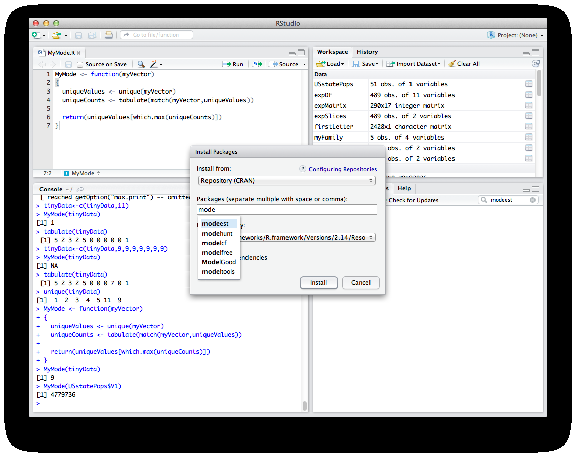
MyMode() function in the script editor, the R console with test output, and the Install Packages dialog for finding the modeest package.
