Section 18.3 Running the Apriori Algorithm
Now we can prepare to generate some rules with the
apriori() command. The term "apriori" refers to the specific algorithm that R will use to scan the data set for appropriate rules. Apriori is a very commonly used alrgorithm and it is quite efficient at finding rules in transaction data. Rules are in the form of "if LHS then RHS." The acronym LHS means "left hand side" and, naturally, RHS means "right hand side." So each rule states that when the thing or things on the left hand side of the equation occur(s), the thing on the right hand side occurs a certain percentage of the time. To reiterate a definition provided earlier in the chapter, support for a rule refers to the frequency of co-occurrence of both members of the pair, i.e., LHS and RHS together. The confidence of a rule refers to the proportion of the time that LHS and RHS occur together versus the total number of appearances of LHS. For example, if Milk and Butter occur together in 10% of the grocery carts (that is "support"), and Milk (by itself, ignoring Butter) occurs in 25% of the carts, then the confidence of the Milk/Butter rule is 0.10/0.25 = 0.40.
There are a couple of other measures that can help us zero in on good association rules - such as "lift"and "conviction" - but we will put off discussing these until a little later. One last note before we start using
apriori(): For most of the work the data miners do with association rules, the RHS part of the equation contains just one item, like "Butter." On the other hand, LHS can and will contain multiple items. A simple rule might just have Milk in LHS and Butter in RHS, but a more complex rule might have Milk and Bread together in LHS with Butter in RHS.
In the spirit of experimentation, we can try out some different parameter values for using the
apriori() command, just to see what we will get:
apriori(Groceries,parameter=list(support=0.005,+
confidence=0.5))
parameter specification:

confidence minval smax arem  aval
       0.5    0.1    1 none FALSE

originalSupport support minlen maxlen target   ext
           TRUE   0.005      1     10  rules FALSE


algorithmic control:

filter tree heap memopt load sort verbose
   0.1 TRUE TRUE  FALSE TRUE    2    TRUE

apriori - find association rules with the apriori algorithm

version 4.21 (2004.05.09) (c) 1996-2004 Christian
Borgelt

set item appearances ...[0 item(s)] done [0.00s].

set transactions ...[169 item(s), 9835 transaction(s)] done [0.00s].

sorting and recoding items ... [120 item(s)] done [0.00s].

creating transaction tree ... done [0.01s].

checking subsets of size 1 2 3 4 done [0.01s].

writing ... [120 rule(s)] done [0.00s].

creating S4 object ... done [0.00s].

set of 120 rules
We set up the
apriori() command to use a support of 0.005 (half a percent) and confidence of 0.5 (50%) as the minimums. These values are confirmed in the first few lines of output. Some other confirmations, such as the value of "minval" and "smax" are not relevant to us right now - they have sensible defaults provided by the apriori() implementation. The "minlen" and "maxlen" parameters also have sensible defaults: these refer to the minimum and maximum length of item set that will be considered in generating rules. Obviously you can’t generate a rule unless you have at least one item in an item set, and setting maxlen to 10 ensures that we will not have any rules that contain more than 10 items. If you recall from earlier in the chapter, the average cart only has 4.4 items, so we are not likely to produce rules involving more than 10 items.
In fact, a little later in the
apriori() output above, we see that the apriori() algorithm only had to examine "subsets of size" one, two three, and four. Apparently no rule in this output contains more than four items. At the very end of the output we see that 120 rules were generated. Later on we will examine ways of making sense out of a large number of rules, but for now let’s agree that 120 is too many rules to examine. Let’s move our support to one percent and rerun apriori(). This time we will store the resulting rules in a data structure called ruleset:
ruleset <- apriori(Groceries,
  parameter=list(support=0.01, confidence=0.5))
If you examine the output from this command, you should find that we have slimmed down to 15 rules, quite a manageable number to examine one by one. We can get a preliminary look at the rules using the summary function, like this:
summary(ruleset)
set of 15 rules

rule length distribution (lhs + rhs):sizes
 3
15

Min. 1st Qu. Median Mean 3rd Qu. Max.
   3       3      3    3       3    3

summary of quality measures:

  support          confidence         lift
Min.   :0.01007   Min.   :0.5000  Min.   :1.984
1st Qu.:0.01174   1st Qu.:0.5151  1st Qu.:2.036
Median :0.01230   Median :0.5245  Median :2.203
Mean   :0.01316   Mean   :0.5411  Mean   :2.299
3rd Qu.:0.01403   3rd Qu.:0.5718  3rd Qu.:2.432
Max.   :0.02227   Max.   :0.5862  Max.   :3.030

mining info:
      data ntransactions support confidence
 Groceries          9835    0.01        0.5
Looking through this output, we can see that there are 15 rules in total. Under "rule length distribution" it shows that all 15 of the rules have exactly three elements (counting both the LHS and the RHS). Then, under "summary of quality measures," we have an overview of the distributions of support, confidence, and a new parameter called "lift."
Researchers have done a lot of work trying to come up with ways of measuring how "interesting" a rule is. A more interesting rule may be a more useful rule because it is more novel or unexpected. Lift is one such measure. Without getting into the math, lift takes into account the support for a rule, but also gives more weight to rules where the LHS and/or the RHS occur less frequently. In other words, lift favors situations where LHS and RHS are not abundant but where the relatively few occurrences always happen together.
The larger the value of lift, the more "interesting" the rule may be. Now we are ready to take a closer look at the rules we generated. The
inspect() command gives us the detailed contents of the dta object generated by apriori():
inspect(ruleset)
  lhs                    rhs                  support  confidence     lift
1 {curd,
  yogurt}              => {whole milk}       0.01006609 0.5823529 2.279125
2 {other vegetables,
   butter}             => {whole milk}       0.01148958 0.5736041 2.244885
3 {other vegetables,
   domestic eggs}      => {whole milk}       0.01230300 0.5525114 2.162336
4 {yogurt,
   whipped/sour cream} => {whole milk}       0.01087951 0.5245098 2.052747
5 {other vegetables,
   whipped/sour cream} => {whole milk}       0.01464159 0.5070423 1.984385
6 {pip fruit,
   other vegetables}   => {whole milk}       0.01352313 0.5175097 2.025351
7 {citrus fruit,
   root vegetables}    => {other vegetables} 0.01037112 0.5862069 3.029608
8 {tropical fruit,
   root vegetables}    => {other vegetables} 0.01230300 0.5845411 3.020999
9 {tropical fruit,
   root vegetables}    => {whole milk}       0.01199797 0.5700483 2.230969
10 {tropical fruit,
    yogurt}            => {whole milk}       0.01514997 0.5173611 2.024770
11 {root vegetables,
    yogurt}            => {other vegetables} 0.01291307 0.5000000 2.584078
12 {root vegetables,
    yogurt}            => {whole milk}       0.01453991 0.5629921 2.203354
13 {root vegetables,
    rolls/buns}        => {other vegetables} 0.01220132 0.5020921 2.594890
14 {root vegetables,
    rolls/buns}        => {whole milk}       0.01270971 0.5230126 2.046888
15 {other vegetables,
    yogurt}            => {whole milk}       0.02226741 0.5128806 2.007235
You can see that each of the 15 rules shows the LHS, the RHS, the support, the confidence, and the lift. Rules 7 and 8 have the highest level of lift: the fruits and vegetables involved in these two rules have a relatively low frequency of occurrence, but their support and confidence are both relatively high. Contrast these two rules with Rule 1, which also has high confidence, but which has low support. The reason for this is that milk is a frequently occurring item, so there is not much novelty to that rule. On the other hand, the combination of fruits, root vegetables, and other vegetables suggest a need to find out more about customers whose carts may contain only vegetarian or vegan items.
Now it is possible that we have set our parameters for confidence and support too stringently and as a result have missed some truly novel combinations that might lead us to better insights. We can use a data visualization package to help explore this possibility. The R package called arulesViz has methods of visualizing the rule sets generated by
apriori() that can help us examine a larger set of rules. First, install and library the arulesViz package:
install.packages("arulesViz")
library(arulesViz)
These commands will give the usual raft of status and progress messages. When you run the second command you may find that three or four data objects are "masked." As before, these warnings generally will not compromise the operation of the package.
Now lets return to our
apriori() command, but we will be much more lenient this time in our minimum support and confidence parameters:
ruleset <- apriori(Groceries,
  parameter=list(support=0.005, confidence=0.35))
We brought support back to half of one percent and confidence down to 35%. When you run this command you should find that you now generate 357 rules. That is way too many rules to examine manually, so let’s use the arulesViz package to see what we have. We will use the
plot() command that we have also used earlier in the book. You may ask yourself why we needed to library the arulesViz package if we are simply going to use an old command. The answer to this conundrum is that arulesViz has put some plumbing into place so that when plot runs across a data object of type "rules" (as generated by apriori) it will use some of the code that is built into arulesViz to do the work. So by installing arulesViz we have put some custom visualization code in place that can be used by the generic plot() command. The command is very simple:
plot(ruleset)
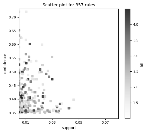
plot(ruleset): a scatter plot of 357 association rules with support on the x-axis, confidence on the y-axis, and lift shown by the shade of each point.Even though we see a two dimensional plot, we actually have three variables represented here. Support is on the X-axis and confidence is on the Y-axis. All else being equal we would like to have rules that have high support and high confidence. We know, however, that lift serves as a measure of interestingness, and we are also interested in the rules with the highest lift. On this plot, the lift is shown by the darkness of a dot that appears on the plot. The darker the dot, the close the lift of that rule is to 4.0, which appears to be the highest lift value among these 357 rules.
The other thing we can see from this plot is that while the support of rules ranges from somewhere below 1% all the way up above 7%, all of the rules with high lift seem to have support below 1%. On the other hand, there are rules with high lift and high confidence, which sounds quite positive.
Based on this evidence, lets focus on a smaller set of rules that only have the very highest levels of lift. The following command makes a subset of the larger set of rules by choosing only those rules that have lift higher than 3.5:
goodrules <- ruleset[quality(ruleset)$lift > 3.5]
Note that the use of the square braces with our data structure ruleset allows us to index only those elements of the data object that meet our criteria. In this case, we use the expression quality(ruleset)$ lift to tap into the lift parameter for each rule. The inequality test > 3.5 gives us just those rules with the highest lift. When you run this line of code you should find that goodrules contins just nine rules. Let’s inspect those nine rules:
inspect(goodrules)
  lhs                     rhs                   support confidence     lift
1 {herbs}              => {root vegetables} 0.007015760  0.4312500 3.956477
2 {onions,
   other vegetables}   => {root vegetables} 0.005693950  0.4000000 3.669776
3 {beef,
   other vegetables}   => {root vegetables} 0.007930859  0.4020619 3.688692
4 {tropical fruit,
   curd}               => {yogurt}          0.005287239  0.5148515 3.690645
5 {citrus fruit,
   pip fruit}          => {tropical fruit}  0.005592272  0.4044118 3.854060
6 {pip fruit,
   other vegetables,
   whole milk}         => {root vegetables} 0.005490595  0.4060150 3.724961
7 {citrus fruit,
   other vegetables,
   whole milk}         => {root vegetables} 0.005795628  0.4453125 4.085493
8 {root vegetables,
   whole milk,
   yogurt}             => {tropical fruit}  0.005693950  0.3916084 3.732043
9 {tropical fruit,
   other vegetables,
   whole milk}         => {root vegetables} 0.007015760  0.4107143 3.768074
There we go again with the microscopic font size. When you look over these rules, it seems evidence that shoppers are purchasing particular combinations of items that go together in recipes. The first three rules really seem like soup! Rules four and five seem like a fruit platter with dip. The other four rules may also connect to a recipe, although it is not quite so obvious what.
The key takeaway point here is that using a good visualization tool to examine the results of a data mining activity can enhance the process of sorting through the evidence and making sense of it. If we were to present these results to a store manager (and we would certainly do a little more digging before formulating our final conclusions) we might recommend that recipes could be published along with coupons and popular recipes, such as for homemade soup, might want to have all of the ingredients group together in the store along with signs saying, "Mmmm, homemade soup!"

