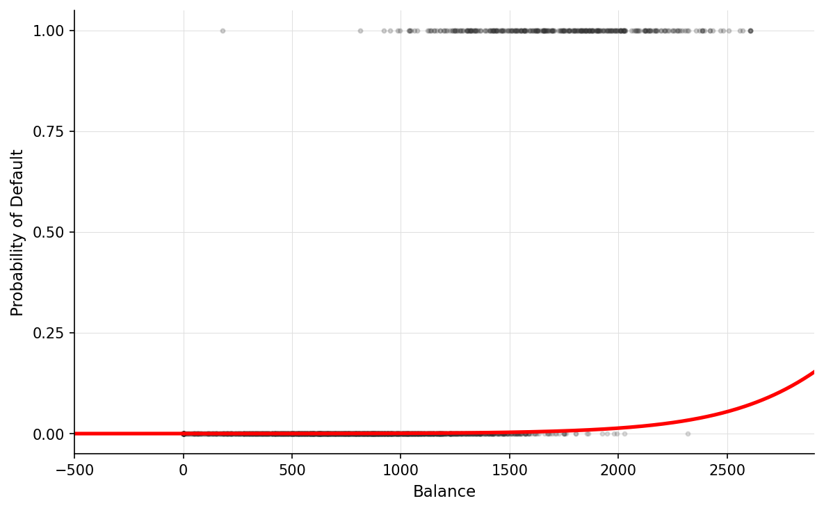
When building a logistic regression model, it is going to look very similar to the linear regression model we built starting in Section 8.7. The major difference from a coding perspective between a linear regression and a logistic regression model is that instead of using lm(), you need to use glm().
Before we create our model, let’s take a step back. Logistic regression, just like linear regression, is a tool to help us predict an outcome. Specifically, we are predicting the probability of an outcome.
where (p) is the probability of default. The left-hand side is called the logit, or log-odds. Notice that the right-hand side looks just like a straight-line regression.
In Linear Regression, your line goes on forever in both directions. But in probability, you can’t be less than 0% or more than 100%. If you used a straight line to predict defaults, the math might eventually say someone has a -20% chance of defaulting, which is impossible.
In the figure above, notice how the red line transitions from a low probability to a high probability as the balance increases. Unlike a straight linear line, this S-curve naturally ’levels off’ at 0 and 1, ensuring our predictions remain realistic probabilities.
# We are using binomial as family since default is yes/no

train_model <- glm(default ~ student + balance + income,
                   family = "binomial", data = training_data)

summary(train_model)
Call:
glm(formula = default ~ student + balance + income, family = "binomial",
    data = training_data)

Coefficients:
              Estimate Std. Error z value Pr(>|z|)
(Intercept) -1.090e+01  5.931e-01 -18.372  < 2e-16 ***
studentYes  -8.245e-01  2.835e-01  -2.908  0.00364 **
balance      5.796e-03  2.805e-04  20.661  < 2e-16 ***
income       2.768e-06  9.736e-06   0.284  0.77614
---
Signif. codes:  0 '***' 0.001 '**' 0.01 '*' 0.05 '.' 0.1 ' ' 1

(Dispersion parameter for binomial family taken to be 1)

    Null deviance: 2043.8  on 6999  degrees of freedom
Residual deviance: 1098.2  on 6996  degrees of freedom
AIC: 1106.2

Number of Fisher Scoring iterations: 8
After we create our model and call summary(), we get an output that should look similar to the outputs we’ve seen before in this chapter. Taking a look at our wall of words, it is incredibly important to note that the numbers here represent the log-odds
While the outputs look the same, there is a major difference in the numbers that are output in a logistic regression vs a linear regression. Remember earlier when we calculated the probability of someone defaulting? It was mentioned that probabilities will always be a number between 0 and 1. But, when we are creating a line in a regression model, we can get any numbers between -∞ and ∞. How does logistic regression, which uses probabilities, make a line then?
We need to get a number that actually has a range, and this is exactly where log-odds come in. Because with regression, we need to get a line (and to build a line, we need a formula). Instead of modeling probability, we model the log of the odds. Here is the step by step of how logistic regression works:
# Convert log-odds → odds ratios
exp(coef(train_model))

# Example: students have 0.43× the odds (≈57% lower odds) of defaulting
 (Intercept)   studentYes      balance       income
1.850225e-05 4.384379e-01 1.005813e+00 1.000003e+00
A very important thing to note is that odds and probability are not the same thing. With odds ratios, we are looking to see how much larger or smaller it is than 1.
If you are a student, the odds of you defaulting decrease, as the odds ratio is 0.438. Their odds are 56.2% lower than non-students (1 - 0.438). This is a significant difference.
For every dollar your balance increases, the odds of you defaulting increase by 0.58%. This seems small per dollar, but compounds rapidly across real-life balance amounts. For example, increasing the balance by $100 multiplies the odds of default by about 1.78, which is a 78% increase in odds.
Unlike in linear regression, logistic regression does not have an R²: (for a review on R²: see Section 8.7). However, we can use the pR2() function from the pscl library ([D.1.21]) to calculate a pseudo R² value.
Just like in Section 7.8, we want to check to see if there is any interactions between some of our variables that may be impacting our regression model. Using the vif() function from the car library ([D.1.2]), we can see the interactions between our variables in our model.