distinct().
Keep only distinct rows from a data frame.
palmerpenguins package. It has the dataset penguins that we are going to use. If you use the helper function and write ?palmerpenguins or ?penguins you will find a description of the data (hint: it’s data related to penguins).
ncol(penguins)      # Finding out the number of columns

nrow(penguins)      # Finding out the number of rows

colnames(penguins)  # Finding out the names of the columns
[1] 8
[1] 344
[1] "species"           "island"            "bill_length_mm"
[4] "bill_depth_mm"     "flipper_length_mm" "body_mass_g"
[7] "sex"               "year"
distinct() function to get this information.
distinct().penguins |> distinct(species)
# A tibble: 3 × 1
  species
  <fct>
1 Adelie
2 Gentoo
3 Chinstrap
penguins dataset. But it doesn’t stop there - you can also use the distinct() command to see distinct combinations of data too. For example:
penguins |> distinct(species, island)
# A tibble: 5 × 2
  species   island
  <fct>     <fct>
1 Adelie    Torgersen
2 Adelie    Biscoe
3 Adelie    Dream
4 Gentoo    Biscoe
5 Chinstrap Dream
select() command!
select().penguins |> select(species, island, bill_length_mm, body_mass_g)
# A tibble: 344 × 4
   species island    bill_length_mm body_mass_g
   <fct>   <fct>              <dbl>       <int>
 1 Adelie  Torgersen           39.1        3750
 2 Adelie  Torgersen           39.5        3800
 3 Adelie  Torgersen           40.3        3250
 4 Adelie  Torgersen           NA            NA
 5 Adelie  Torgersen           36.7        3450
 6 Adelie  Torgersen           39.3        3650
 7 Adelie  Torgersen           38.9        3625
 8 Adelie  Torgersen           39.2        4675
 9 Adelie  Torgersen           34.1        3475
10 Adelie  Torgersen           42          4250
# ℹ 334 more rows
# This is saying let's take the first column, and then every column from 3 to 5
penguins |> select(1,3:5)
# A tibble: 344 × 4
   species bill_length_mm bill_depth_mm flipper_length_mm
   <fct>            <dbl>         <dbl>             <int>
 1 Adelie            39.1          18.7               181
 2 Adelie            39.5          17.4               186
 3 Adelie            40.3          18                 195
 4 Adelie            NA            NA                  NA
 5 Adelie            36.7          19.3               193
 6 Adelie            39.3          20.6               190
 7 Adelie            38.9          17.8               181
 8 Adelie            39.2          19.6               195
 9 Adelie            34.1          18.1               193
10 Adelie            42            20.2               190
# ℹ 334 more rows
==: Equal to!=: Not equal to>=: Greater than or equal to<=: Less than or equal to>: Greater than<: Less than&: And|: Or%in%: Withinselect() command. But, when we want to filter the data inside a dataset, we utilize the filter() command.
filter().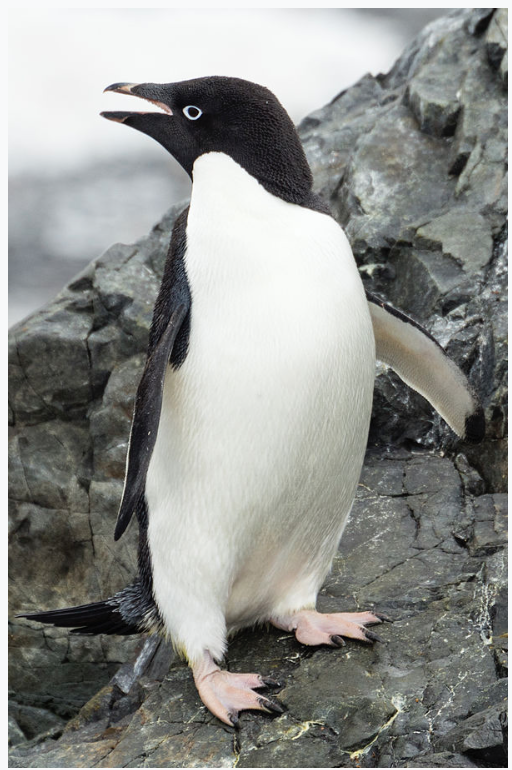
penguins |>
  filter(species == "Adelie")
# A tibble: 152 × 8
   species island    bill_length_mm bill_depth_mm flipper_length_mm body_mass_g
   <fct>   <fct>              <dbl>         <dbl>             <int>       <int>
 1 Adelie  Torgersen           39.1          18.7               181        3750
 2 Adelie  Torgersen           39.5          17.4               186        3800
 3 Adelie  Torgersen           40.3          18                 195        3250
 4 Adelie  Torgersen           NA            NA                  NA          NA
 5 Adelie  Torgersen           36.7          19.3               193        3450
 6 Adelie  Torgersen           39.3          20.6               190        3650
 7 Adelie  Torgersen           38.9          17.8               181        3625
 8 Adelie  Torgersen           39.2          19.6               195        4675
 9 Adelie  Torgersen           34.1          18.1               193        3475
10 Adelie  Torgersen           42            20.2               190        4250
# ℹ 142 more rows
# ℹ 2 more variables: sex <fct>, year <int>
filter() command, we can have as many conditions as possible. One incredibly important decision is whether to use and/or.
& symbol.
penguins |>
  filter(species == "Adelie" & island == "Torgersen")
# A tibble: 52 × 8
   species island    bill_length_mm bill_depth_mm flipper_length_mm body_mass_g
   <fct>   <fct>              <dbl>         <dbl>             <int>       <int>
 1 Adelie  Torgersen           39.1          18.7               181        3750
 2 Adelie  Torgersen           39.5          17.4               186        3800
 3 Adelie  Torgersen           40.3          18                 195        3250
 4 Adelie  Torgersen           NA            NA                  NA          NA
 5 Adelie  Torgersen           36.7          19.3               193        3450
 6 Adelie  Torgersen           39.3          20.6               190        3650
 7 Adelie  Torgersen           38.9          17.8               181        3625
 8 Adelie  Torgersen           39.2          19.6               195        4675
 9 Adelie  Torgersen           34.1          18.1               193        3475
10 Adelie  Torgersen           42            20.2               190        4250
# ℹ 42 more rows
# ℹ 2 more variables: sex <fct>, year <int>
& symbol, we need to use the | symbol.
penguins |>
  filter(species == "Adelie" | island == "Torgersen")
# A tibble: 152 × 8
   species island    bill_length_mm bill_depth_mm flipper_length_mm body_mass_g
   <fct>   <fct>              <dbl>         <dbl>             <int>       <int>
 1 Adelie  Torgersen           39.1          18.7               181        3750
 2 Adelie  Torgersen           39.5          17.4               186        3800
 3 Adelie  Torgersen           40.3          18                 195        3250
 4 Adelie  Torgersen           NA            NA                  NA          NA
 5 Adelie  Torgersen           36.7          19.3               193        3450
 6 Adelie  Torgersen           39.3          20.6               190        3650
 7 Adelie  Torgersen           38.9          17.8               181        3625
 8 Adelie  Torgersen           39.2          19.6               195        4675
 9 Adelie  Torgersen           34.1          18.1               193        3475
10 Adelie  Torgersen           42            20.2               190        4250
# ℹ 142 more rows
# ℹ 2 more variables: sex <fct>, year <int>
==, as we have other options. Below are two options: the first filters for any body mass over 4,000 grams, and the second filters for species that are either Adelie or Gentoo.
penguins |> filter(body_mass_g >= 4000)
# A tibble: 177 × 8
   species island    bill_length_mm bill_depth_mm flipper_length_mm body_mass_g
   <fct>   <fct>              <dbl>         <dbl>             <int>       <int>
 1 Adelie  Torgersen           39.2          19.6               195        4675
 2 Adelie  Torgersen           42            20.2               190        4250
 3 Adelie  Torgersen           34.6          21.1               198        4400
 4 Adelie  Torgersen           42.5          20.7               197        4500
 5 Adelie  Torgersen           46            21.5               194        4200
 6 Adelie  Dream               39.2          21.1               196        4150
 7 Adelie  Dream               39.8          19.1               184        4650
 8 Adelie  Dream               44.1          19.7               196        4400
 9 Adelie  Dream               39.6          18.8               190        4600
10 Adelie  Dream               42.3          21.2               191        4150
# ℹ 167 more rows
# ℹ 2 more variables: sex <fct>, year <int>
penguins |> filter(species %in% c("Adelie", "Gentoo"))
# A tibble: 276 × 8
   species island    bill_length_mm bill_depth_mm flipper_length_mm body_mass_g
   <fct>   <fct>              <dbl>         <dbl>             <int>       <int>
 1 Adelie  Torgersen           39.1          18.7               181        3750
 2 Adelie  Torgersen           39.5          17.4               186        3800
 3 Adelie  Torgersen           40.3          18                 195        3250
 4 Adelie  Torgersen           NA            NA                  NA          NA
 5 Adelie  Torgersen           36.7          19.3               193        3450
 6 Adelie  Torgersen           39.3          20.6               190        3650
 7 Adelie  Torgersen           38.9          17.8               181        3625
 8 Adelie  Torgersen           39.2          19.6               195        4675
 9 Adelie  Torgersen           34.1          18.1               193        3475
10 Adelie  Torgersen           42            20.2               190        4250
# ℹ 266 more rows
# ℹ 2 more variables: sex <fct>, year <int>
is.na() to filter for which are NA and the drop_na() to remove all rows that have at least one NA value.
penguins |> filter(is.na(body_mass_g)) # Filter for rows that have missing data
# A tibble: 2 × 8
  species island    bill_length_mm bill_depth_mm flipper_length_mm body_mass_g
  <fct>   <fct>              <dbl>         <dbl>             <int>       <int>
1 Adelie  Torgersen             NA            NA                NA          NA
2 Gentoo  Biscoe                NA            NA                NA          NA
# ℹ 2 more variables: sex <fct>, year <int>
penguins |> drop_na(body_mass_g) # Filters for rows that don't have missing data
# A tibble: 342 × 8
   species island    bill_length_mm bill_depth_mm flipper_length_mm body_mass_g
   <fct>   <fct>              <dbl>         <dbl>             <int>       <int>
 1 Adelie  Torgersen           39.1          18.7               181        3750
 2 Adelie  Torgersen           39.5          17.4               186        3800
 3 Adelie  Torgersen           40.3          18                 195        3250
 4 Adelie  Torgersen           36.7          19.3               193        3450
 5 Adelie  Torgersen           39.3          20.6               190        3650
 6 Adelie  Torgersen           38.9          17.8               181        3625
 7 Adelie  Torgersen           39.2          19.6               195        4675
 8 Adelie  Torgersen           34.1          18.1               193        3475
 9 Adelie  Torgersen           42            20.2               190        4250
10 Adelie  Torgersen           37.8          17.1               186        3300
# ℹ 332 more rows
# ℹ 2 more variables: sex <fct>, year <int>
arrange() command allows us to organize our data very nicely. There are only two options: ascending or descending order. By default, arrange() orders the data in ascending order.
arrange().penguins |> arrange(body_mass_g) # ascending order
# A tibble: 344 × 8
   species   island   bill_length_mm bill_depth_mm flipper_length_mm body_mass_g
   <fct>     <fct>             <dbl>         <dbl>             <int>       <int>
 1 Chinstrap Dream              46.9          16.6               192        2700
 2 Adelie    Biscoe             36.5          16.6               181        2850
 3 Adelie    Biscoe             36.4          17.1               184        2850
 4 Adelie    Biscoe             34.5          18.1               187        2900
 5 Adelie    Dream              33.1          16.1               178        2900
 6 Adelie    Torgers…           38.6          17                 188        2900
 7 Chinstrap Dream              43.2          16.6               187        2900
 8 Adelie    Biscoe             37.9          18.6               193        2925
 9 Adelie    Dream              37.5          18.9               179        2975
10 Adelie    Dream              37            16.9               185        3000
# ℹ 334 more rows
# ℹ 2 more variables: sex <fct>, year <int>
penguins |> arrange(desc(body_mass_g)) # descending order
# A tibble: 344 × 8
   species island bill_length_mm bill_depth_mm flipper_length_mm body_mass_g
   <fct>   <fct>           <dbl>         <dbl>             <int>       <int>
 1 Gentoo  Biscoe           49.2          15.2               221        6300
 2 Gentoo  Biscoe           59.6          17                 230        6050
 3 Gentoo  Biscoe           51.1          16.3               220        6000
 4 Gentoo  Biscoe           48.8          16.2               222        6000
 5 Gentoo  Biscoe           45.2          16.4               223        5950
 6 Gentoo  Biscoe           49.8          15.9               229        5950
 7 Gentoo  Biscoe           48.4          14.6               213        5850
 8 Gentoo  Biscoe           49.3          15.7               217        5850
 9 Gentoo  Biscoe           55.1          16                 230        5850
10 Gentoo  Biscoe           49.5          16.2               229        5800
# ℹ 334 more rows
# ℹ 2 more variables: sex <fct>, year <int>
$ symbol. In tidyverse, we can also create new columns, but instead of using the $, we can use the mutate() command.
mutate().# Base R
penguins$bill_ratio <- penguins$bill_length_mm / penguins$bill_depth_mm
penguins <- penguins |>
mutate(bill_ratio = bill_length_mm / bill_depth_mm)
if_else() or case_when() command.
if_else() where we first add the criteria we want to build a column using, the value if it fits the criteria, and the value if it does not fit the criteria.
penguins |>
  mutate(size_category = if_else(body_mass_g >= 3500, "Big","Small"))
# A tibble: 344 × 10
   species island    bill_length_mm bill_depth_mm flipper_length_mm body_mass_g
   <fct>   <fct>              <dbl>         <dbl>             <int>       <int>
 1 Adelie  Torgersen           39.1          18.7               181        3750
 2 Adelie  Torgersen           39.5          17.4               186        3800
 3 Adelie  Torgersen           40.3          18                 195        3250
 4 Adelie  Torgersen           NA            NA                  NA          NA
 5 Adelie  Torgersen           36.7          19.3               193        3450
 6 Adelie  Torgersen           39.3          20.6               190        3650
 7 Adelie  Torgersen           38.9          17.8               181        3625
 8 Adelie  Torgersen           39.2          19.6               195        4675
 9 Adelie  Torgersen           34.1          18.1               193        3475
10 Adelie  Torgersen           42            20.2               190        4250
# ℹ 334 more rows
# ℹ 4 more variables: sex <fct>, year <int>, bill_ratio <dbl>,
#   size_category <chr>
if_else(). But, when there are three or more criteria, we can use the case_when() command. Instead of having just “Big” and “Small”, let’s add the category “Gigantic”.
penguins |>
  mutate(size_category = case_when(
    body_mass_g <= 3500 ~ "Small",
    body_mass_g > 3500 & body_mass_g <= 4000 ~ "Big",
    body_mass_g > 4000 ~ "Gigantic",
    TRUE ~ "Unknown"   # catch-all for NAs or anything else
  ))
# A tibble: 344 × 10
   species island    bill_length_mm bill_depth_mm flipper_length_mm body_mass_g
   <fct>   <fct>              <dbl>         <dbl>             <int>       <int>
 1 Adelie  Torgersen           39.1          18.7               181        3750
 2 Adelie  Torgersen           39.5          17.4               186        3800
 3 Adelie  Torgersen           40.3          18                 195        3250
 4 Adelie  Torgersen           NA            NA                  NA          NA
 5 Adelie  Torgersen           36.7          19.3               193        3450
 6 Adelie  Torgersen           39.3          20.6               190        3650
 7 Adelie  Torgersen           38.9          17.8               181        3625
 8 Adelie  Torgersen           39.2          19.6               195        4675
 9 Adelie  Torgersen           34.1          18.1               193        3475
10 Adelie  Torgersen           42            20.2               190        4250
# ℹ 334 more rows
# ℹ 4 more variables: sex <fct>, year <int>, bill_ratio <dbl>,
#   size_category <chr>
rename() command.
rename() command is:.penguins |> rename(penguin_types = species)
# A tibble: 344 × 9
   penguin_types island    bill_length_mm bill_depth_mm flipper_length_mm
   <fct>         <fct>              <dbl>         <dbl>             <int>
 1 Adelie        Torgersen           39.1          18.7               181
 2 Adelie        Torgersen           39.5          17.4               186
 3 Adelie        Torgersen           40.3          18                 195
 4 Adelie        Torgersen           NA            NA                  NA
 5 Adelie        Torgersen           36.7          19.3               193
 6 Adelie        Torgersen           39.3          20.6               190
 7 Adelie        Torgersen           38.9          17.8               181
 8 Adelie        Torgersen           39.2          19.6               195
 9 Adelie        Torgersen           34.1          18.1               193
10 Adelie        Torgersen           42            20.2               190
# ℹ 334 more rows
# ℹ 4 more variables: body_mass_g <int>, sex <fct>, year <int>,
#   bill_ratio <dbl>
tidyverse to the test and perform our functions together!
penguins_new <- penguins |>
  select(species, island, bill_length_mm, body_mass_g) |>
  filter(species == "Adelie") |>
  mutate(size_category = if_else(body_mass_g >= 3500, "Big","Small")) |>
  arrange(desc(body_mass_g)) |>
  rename(penguin_types = species)
penguins_new is the name of the new dataset.<- commandpenguins
tidyverse.

